Download
1 / 71
710 likes | 803 Views
Learn about the motivation behind multimedia compression techniques for images, audio, and video. Explore coding redundancy and psycho-visual redundancy in image compression. Understand how quantization is used to reduce data size.

E N D
Multimedia Compression - 1
Content • Motivation • Compression Techniques • Image Compression • JPEG
Motivation Text: • 1 page with 80 char/line and 64 lines/page and 2 Byte/Char • 80 x 64 x 2 x 8 = 80 kBit/page Image: • 24 Bit/Pixel, 512 x 512 Pixel/image • 512 x 512 x 24 = 6 MBit/Image Audio: • CD-quality, samplerate44,1 kHz, 16 Bit/sample • Mono: 44,1 x 16 = 706 kBit/s Stereo: 1.412 MBit/s Video: • full frames with 1024 x 1024 Pixel/frame, 24 Bit/Pixel, 30 frames/s 1024 x 1024 x 24 x 30 = 720 MBit/s • more realistic 360 x 240 Pixel/frame = 60 MBit/s Hence compression is NECESSARY
Compression • Coding of data to minimize its representation • reduce the storage requirement • increase the communication rate • reduce redundancy prior to encryption (security) • Different techniques for • each type of object, and • each type of media • Technique must be • fast, one-pass and adaptive • invertible, and impose reasonable memory requirements.
Image Compression Images can be compressed by exploiting two characteristics of digital images Redundancy • coding redundancy • Inter-pixel redundancy Irrelevancy (Psycho-visual redundancy) • Much of the data in an image may be irrelevant to a human observer
Image Compression Coding redundancy: it is a mathematically quantifiable entity and is transforming a 2D pixel array into a statistical uncorrelated data set. In 1940s Shannon firs formulated the probabilistic view of information and its representation, transmission and compression. I(E) = log(1/P(E))
Image Compression Example: Let n1, and n2 the number of data in two data sets that represent the same information. The relative data redundancy RD of the first data set RD = 1 – 1/CR where CR = n1/n2 compression ratio If n2 = n1, CR = 1; RD = 0 If n2 << n1, CR; RD 1 If n2 >> n1, CR 0; RD - In general CR (0, ) RD (- , 1)
Image Compression- Coding Redundancy Great deal of information about the appearance of an image could be obtained form a histogram of its gray levels. Gray level histogram (graph of pr(rk) against rk) of an image can provide a great deal of insight into the construction of codes to reduce the amount of data used to represent it.
Image Compression- Coding Redundancy pr(rk) = nk/n k = 0, 1, 2, . . ., L-1 ; n = total number of pixels L= number of gray levels rk : discrete random variable in the interval 0, 1 that represents gray levels of an image. pr(rk): probability that each (rk) occurs l (rk): number of bits used to represent each value of rk Average length of code:Lavg =SUM( l (rk) pr(rk) )
Image Compression- Coding Redundancy Example: 8-level image has distribution as shown
Image Compression- Coding Redundancy Lavg = SUM( l (rk) pr(rk)) = 2(0.19) + 2(0.25) + 2(0.21) + . . . +6(0.02) = 2.7 bits for code 2 Lavg = 3 bits for code 1 (%10 of data is redundant) CR = 3 / 2.7 or 1.11 RD = 1 - 1/1.11 = 0.099
Image Compression- Psycho-visual Redundancy • The eye does not respond with equal sensitivity to all visual information. Some information has less relative importance than others. This information is said to be psycho-visually redundant. • Its elimination is possible only because the information itself is not essential for normal visual processing.
Image Compression- Psycho-visual Redundancy • Elimination of psycho-visually redundant data results in a loss of quantitative information, it is commonly referred to as quantization. • Quantization is mapping of a broad range of input values to a limited number of output values. • It is an irreversible operation that results in lossy data compression
Image Compression- Psycho-visual Redundancy Gray Scale (GS) quantization: An 8-bit monochrome image can be quantized to 4-bit image False contours appear due to coarse quantization
Image Compression- Psycho-visual Redundancy • Improved Gray Scale (IGS) quantization: • It recognizes the eye’s inherent sensitivity to edges and breaks them up by adding to each pixel a pseudo random number, which is generated form the low order bits of neighboring pixels, before quantizing the result. • Procedure for quantization: • sum is initially set to zero • current 8-bit gray code is added to the least significant four bits of the previously generated sum. If the four most significant bits of the current pixel is 1111, 0000 is added. • the four most significant bits of the sum is used as IGS code
Image Compression- Psycho-visual Redundancy Gonzales, Woods.Digital Image Processing, pp. 318
Image Compression- Psycho-visual Redundancy GS Quantization IGS Quantization Gonzales, Woods.Digital Image Processing, pp. 317
Fidelity Criteria Because information of interest may be lost as a result of quantization, quantifying the nature and extent of information lost is important Objective Fidelity Criteria Information lost is expressed in terms of original image and the compressed image. Root-mean-square error between an input and output image Let f(x, y) represent an input image f^(x, y) approximation of f(x, y) e(x, y) = f^ (x, y) - f(x, y)
Fidelity Criteria for M X N image
Compression Techniques Lossy (noisy) techniques vs. lossless techniques Lossless compression • assumes every bit of information is important • original object can be perfectly recovered • Compression ratios • 2:1 average for text • 15:1 Black and White images
Compression Techniques Lossy compression • assumes some of the data is unnecessary • humans cannot notice the difference between the original object and the decompressed object • Compression ratios • 50:1 average • 200:1 goal
Entropy Coding • An efficient method for coding • Encode frequent events with fewer bits • Assign shorter code words to objects that occur more frequently. • Generally used in conjunction with other techniques • Very common
Entropy Coding: Principal • example: given 4 possible symbols (words) in source code • IF all equal p=1/4: H(P)=2; • IF p= 1/2, 1/4, 1/8, 1/8 --> H(P)= 1.75
Huffman Coding Basics: • Assumption: some symbols occur more often than others • E.g., character frequencies of the English language • Idea: frequent symbols --> shorter bit strings (cf. Entropy!) Example: • Characters to be encoded: A, B, C, D, E • probability to occur: p(A)=0.3, p(B)=0.3, p(C)=0.1, p(D)=0.15, p(E)=0.15
Arithmetic Coding • Arithmetic coding is a more modern coding method that usually out-performs Huffman coding. • Huffman coding assigns each symbol a codeword which has an integral bit length. Arithmetic coding can treat the whole message as one unit. • A message is represented by a half-open interval [a, b) where a and b are real numbers between 0 and 1. Initially, the interval is [0, 1). When the message becomes longer, the length of the interval shortens and the number of bits needed to represent the interval increases. Li & Drew 27
Arithmetic Coding Example to arithmetic coding Encode the following stream of characters using decimal arithmetic codingcompression: MEDIA You may assume that characters occur with probabilities of M = 0.1, E = 0.3, D = 0.3, I = 0.2 and A = 0.1.
Arithmetic Coding Sort Data into largest probabilities first and make cumulative probabilities 0 - E - 0.3 - D - 0.6 – I – 0.8 – M - 0.9 – A – 1.0 There are only 5 Characters so there are 5 segments of width determined by theprobability of the related character.
Arithmetic Coding The first character to encoded is M which is in the range 0.8 – 0.9, therefore the rangeof the final codeword is in the range 0.8 to 0.89999….. Each subsequent character subdivides the range 0.8 – 0.9 SO after coding M we get 0.8 - E - 0.83 - D - 0.86 – I – 0.88 – M - 0.89 – A – 0.9
Arithmetic Coding So to code E we get range 0.8 – 0.83 SO we subdivide this range (.03) 0.8 - E - 0.809 - D - 0.818 – I – 0.824 – M - 0.827 – A – 0.83 Next range is for D so we split in the range 0.809 – 0.818 (.009) 0.809 - E - 0.8117 - D - 0.8144 – I – 0.8162 – M - 0.8171 – A – 0.818 Next Character is I so range is from 0.8144 – 0.8162 (.0018) so we get 0.8144 - E - 0.81494 - D - 0.81548 – I – 0.81584 – M - 0.81602 –A – 0.8162
Arithmetic Coding Final Char is A which is in the range 0.81602 – 0.8162 So the completed codeword is any number in the range 0.81602 <= codeword < 0.8162
Arithmetic Coding Encoding Assume Codeword is 0.8161 Code can readily determine first character is M since it is in the Range 0.8 – 0.9 By expanding interval we can see that next char must be an E as it is in the range 0.8 –0.83 and so on for all other intervals.
Run Length Encoding • Run length encoding is simple, and very common • Depends on inter pixel redundancy • Look for long sequences of objects with equal value • Pixels of the same intensity • sequence of equal characters • … • Represent by value-count • The longer the sequence, the more savings
Run Length Encoding • The sequence of image elements x1,x2,…,xn is mapped into a sequence of pairs (v1,l1), (v2,l2), …, (vk,lk), where vi represents a value and li the length of the ith run. • Example: 11111111111333333333322222222211111 is represented by (1,11), (3,10), (2,9), (1,5)
Repetition Suppression • A series of n successive occurrences of a specific character is replaced by a special character (e.g. 0 or blank) called flag, followed by a number representing the repetition count. • Example: Zero suppression 98400000000000000000000000000000000 is substituted with 984f32
Pattern Substitution • A shorter code substitutes a frequently occurring pattern. • Example This book is an exemplary example of a book on multimedia and networking. Nowhere else will you find this kind of coverage and completeness. This is truly a one-stop-shop for all that you want to know about multimedia and networking.
Pattern Substitution a, about, all, an, and, for, is, of, on, that, this, to, will, multimedia, networking 1 2 3 4 5 6 7 8 9 + & = # m* n* & b o o k 7 4 e x e m p l a r y e x a m p l e 8 1 b o o k 9 m * 5 n * . N o w h e r e sp e l s e # y o u sp f i n d & k i n d 8 c o v e r a g e 5 c o m p l e t e n e s s . & 7 t r u l y 1 o n e - s t o p - s h o p 6 3 + y o u sp w a n t = k n o w 2 m * 5 n
Source Coding DPCM = Differential Pulse-Code Modulation Assumptions: • Consecutive samples or frames have similar values • Prediction is possible due to existing correlation Fundamental Steps: • Incoming sample or frame (pixel or block) is predicted by means of previously processed data • Difference between incoming data and prediction is determined • Difference is quantized Challenge: optimal predictor • Examples: • Differential pulse code modulation • Delta modulation • Adaptive pulse code modulation
Transform Coding • The raw data undergoes a mathematical transformation from the original form in spatial or temporal domain into an abstract domain,which is more suitable for compression. • The transform process is a reversible process and the original signal can be obtained by applying the inverse transform. • Transformer applies a one-to-one transformation to the input image data. Its output is a representation that is more amenable to compression.
Transform Coding • In image coding, we use a transformation to go from the pixel domain into spatial frequency domain so that the bulk of information is stored in fewer number of bits or a lesser range. • Based on Fourier Transform • Examples: • Cosine Transforms: Amplitudes or intensities are represented by DCT coefficients. • Discrete Cosine Transform (DCT) • Forward DCT (FDCT) • Inverse DCT (IDCT) • Wavelet Transform
Transform Coding … made simple Consider a 2x2 block of monochrome pixels. Suppose we do the following: • Take the value of A as the base value for the transform. This is one of the transform values. • Calculate three other transform values by taking the difference between the three other pixels and pixel A. TRANSFORM INVERSE TRANSFORM x0 = A An = x0 x1 = B - A Bn = x1 + x0 x2 = C - A Cn = x2 + x0 x3 = D - A Dn = x3 + x0
Transform Coding … made simple • At 8 bits per pixel, without transform we need 32 bits for this block. • With transform, we may assign 4 bits for difference values. Thus 8 + (3*4) = 20 or 5 bits per pixel. Transform coding is much more effective with larger blocks.
The JPEG Standard • JPEG is an image compression standard that was developed by the “Joint Photographic Experts Group”. JPEG was formally accepted as an international standard in 1992. • JPEG is a lossy image compression method. It employs a transform coding method using the DCT (Discrete Cosine Transform). • An image is a function of i and j (or conventionally x and y) in the spatial domain. The 2D DCT is used as one step in JPEG in order to yield a frequency response which is a function F(u, v) in the spatial frequency domain, indexed by two integers u and v. Li & Drew 44
Observations for JPEG Image Compression • The effectiveness of the DCT transform coding method in JPEG relies on 3 major observations: Observation 1: Useful image contents change relatively slowly across the image, i.e., it is unusual for intensity values to vary widely several times in a small area, for example, within an 8×8 image block. • much of the information in an image is repeated, hence “spatial redundancy”. 45 Li & Drew
Observations for JPEG Image Compression(cont’d) Observation 2: Psychophysical experiments suggest that humans are much less likely to notice the loss of very high spatial frequency components than the loss of lower frequency components. the spatial redundancy can be reduced by largely reducingthe high spatial frequency contents. Observation 3: Visual acuity (accuracy in distinguishing closely spaced lines) is much greater for gray (“black and white”) than for color. chroma subsampling (4:2:0) is used in JPEG. 46 Li & Drew
JPEG Compression Steps MCU: Minimum Coded Unit FDCT: Forward Discrete Cosine Transformation
Image Preparation • 8x8 pixel blocks (data units)
JPEG Coding Decoding: The same… in reverse!
DCT & Quantization in JPEG The original signal F = f(x,y)