Download
1 / 31
310 likes | 326 Views
Explore estimating dose-response function through the Generalized Propensity Score (GPS) in this talk by Barbara Guardabascio and Marco Ventura from the Italian National Institute of Statistics. They discuss motivations, literature references, and their contributions, explaining the econometrics of dose-response and implementation methods for various treatments. Learn about their programs and applications in assessing public policy program effectiveness with continuous treatment exposure.

E N D
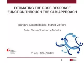
ESTIMATING THE DOSE-RESPONSE FUNCTION THROUGH THE GLM APPROACH Barbara Guardabascio, Marco Ventura Italian National InstituteofStatistics 7th June 2013, Potsdam
Outline of the talk • Motivations; • literature references; • our contribution to the topic; • the econometrics of the dose-response; • how to implement the dose-response; • our programs; • applications.
Motivations • Main question: • how effective are public policy programs with continuous treatment exposure? • Fundamental problem: • treated individuals are self-selected and not randomly. • Treatment is not randomly assigned • (possible) solution: • estimating a dose-response function
Motivations • What is a dose-response function? • It is a relationship between treatment and an outcome variable e.g.: birth weight, employment, bank debt, etc
Motivations • How can we estimate a dose-response function? • It can be estimated by using the Generalized Propensity Score (GPS)
Literature references • Propensity Score for binary treatments: • Rosenbaum and Rubin (1983), (1984) 2. for categorical treatment variables: Imbens (2000), Lechner (2001) 3. Generalized Propensity Score for continuous treatments: Hirano and Imbens, 2004; Imai and Van Dyk (2004)
Our contribution • Ad hoc programs have been provided to STATA users (Bia and Mattei, 2008), but … • … these programs contemplate only Normal distribution of the treatment variable • (gpscore.ado and doseresponse.ado) • We provide new programs to accommodate other distributions, not Normal. • (gpscore2.ado and doseresponse2.ado)
The econometrics of the dose-response • {Yi(t)} set of potential outcomes for • Where is the set of potential treatments over • [t0, t1]
The econometrics of the dose-response Let us suppose to have N individuals, i=1 … N Xi vector of pre-treatment covariates; Ti level of treatment delivered; Yi (Ti) outcome corresponding to the treatment Ti
The econometrics of the dose-response • We want the average dose response function • Hirano-Imbens define the GPS as the conditional density of the actual treatment given the covariates
The econometrics of the dose-response • Balancing property: Within strata with the same r(t,x) the probability that T=t does not depend on X
The econometrics of the dose-response • If weak unconfoundedness holds we have This means that the GPS can be used to eliminate any bias associated with differences in the covariates and …
The econometrics of the dose-response • The dose-response function can be computed as:
How to implement the GPS • The dose-respone can be implemented in 3 steps: FIRST STEP: • Regress Ti on Xi and take the conditional distribution of the treatment given the covariates Ti| Xi
How to implement the GPS Where f(.) is a suitable transformation of T (link) D is a distribution of the exponential family β parameters to be estimated σ conditional SE of T|X
How to implement the GPS GPS 1a. Test the balancing property
How to implement the GPS SECOND STEP: Model the conditional expectation of E[Yi| Ti, Ri ] as a function of Ti and Ri
How to implement the GPS THIRD STEP: Estimate the dose-response function by averaging the estimated conditionl expectation over the GPS at each level of the treatment we are interested in
How to implement the GPS • Where is the novelty? in the FIRST STEP • Instead of a ML we use a GLM • exponential distribution (family) • combined with a link function
our programs • We have written two programs: • doserepsonse2.ado; • estimates the dose-response function and graphs the result. • It carries out step 1 – 2 – 3 of the previous slides by running other 2 programs
our programs • gpscore2.ado: • evaluates the gpscore under 6 different distributional assumptions • step 1 of the previous slides • doseresponse_model.ado: • Carries out step 2 of the previous slides
our programs doseresponse2varlist , outcome(varname) t(varname) family(string) link(string) gpscore(newvarname) predict(newvarname) sigma(newvarname) cutpoints(varname) nq_gps(#) index(string) dose_response(newvarlist) Options t_transf(transformation) normal_test(test) normal_level(#) test_varlist(varlist) test(type) flag(#) cmd(regression_cmd) reg_type_t(string) reg_type_gps(string) interaction(#) t_points(vector) npoints(#) delta(#) bootstrap(string) filename(filename) boot_reps(#) analysis(string) analysis_leve(#) graph(filename) flag_b(#) opt_nb(string) opt_b(varname) detail
our programs gpscore2varlist , t(varname) family(string) link(string) gpscore(newvarname) predict(newvarname) sigma(newvarname) cutpoints(varname) index(string) nq_gps(#) Options t_transf(transformation) normal_test(test) normal_level(#) test_varlist(varlist) test(type) flag_b(#) opt_nb(string) opt_b(varname) detail
Application Data set byImbens, Rubin and Sacerdote (2001); The winnersof a lottery in Massachussets: amountof the prize (treatment) Ti earnings 6 yearsafterwinning (outcome) Yi age, gender, education, # ofticketsbought, working status, earningsbeforewinning up to 6 Xi
Application: flogit Fractional data: flogit model. Treatment: prize/max(prize) outcome: earnings after 6 year family(binomial) link(logit)
Application: count data Count data: Poisson model. Treatment: years of college+ high school outcome: earnings after 6 year family(poisson) link(log)
Application: gamma distribution Gamma distribution: Treatment: age outcome: earnings after 6 year family(gamma) link(log)