Differential Equations:

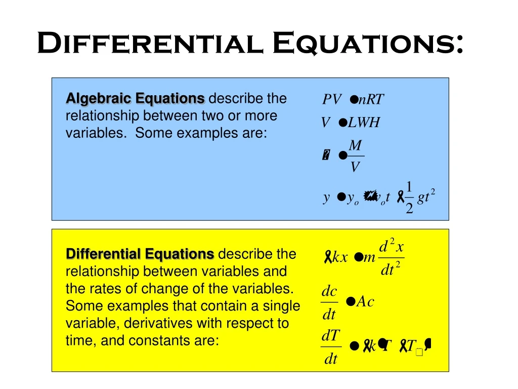
1. Algebraic Equations describe the relationship between two or more variables. Some examples are: Differential Equations describe the relationship between variables and the rates of change of the variables. Some examples that contain a single variable, derivatives with respect to time, and constants are: Differential Equations:

2. Where Do Differential Equations Come From? Differential equations, like algebraic equations, describe relationships that scientists, engineers, economists, entrepreneurs, doctors, etc. encounter every day! Whenever you are interested in how something changes … you are considering a situation where a differential equation applies. • Motion • Heat Up/Cool Down • Charging/Discharging of a Capacitor • Growth/Decay • Population Dynamics • Chemical Concentrations • Stock Market Fluctuations • Many Others!

3. Case #4: Predator/Prey Model Suppose populations of rabbits and foxes are interacting in a simple two species ecosystem. The rabbits have an infinite supply of food and the foxes have no predators. The Lotka-Volterra model is a relatively simple model that demonstrates some tremendously interesting behavior. R(t) is the number of rabbits and F(t) is the number of foxes as functions of time. The parameters are defined as follows: a is the natural growth rate of rabbits in the absence of predation, b is the death rate per encounter of rabbits due to predation, c is the biological efficiency of turning predated rabbits into foxes, d is the natural death rate of foxes in the absence of food (rabbits).

4. Analytic Analysis: Governing Equations: Step 1: look for conditions where R(t) and F(t) match situations we have seen before: This tells us that if foxes do not eat rabbits, then the rabbit population grows exponentially and the fox population dies off exponentially … which makes sense given the assumptions of the model.

5. Step 2: Explore what effect foxes eating rabbits will have on the model: • It will counteract the growth of the rabbit population • It will counteract the decline of the fox population • If there is a high number of rabbits and foxes, the rabbit population will decline and the fox population will grow Step 3: look for conditions where R(t) and F(t) can be constant (that is, situations where dR/dt=0 and dF/dt=0:

6. Numerical Analysis: Use a calculus-based computer model (written using excel) and some values for the constants to explore the details of the model predictions. Case A: a=0.2, b=0, c=0, d=0.1, R(0)=10, F(0)=10: As anticipated … the rabbit population grows exponentially and the fox population dies off exponentially.

7. Case B: a=2.0, b=0.25, c=0.1, d=1.0, R(0)=10, F(0)=8: As anticipated … the initial values of 10 rabbits and 8 foxes yields a steady solution, whereby dR/dt and dF/dt are both equal to zero.

8. Case C: a=2.0, b=0.25, c=0.1, d=1.0, R(0)=10, F(0)=10: The initial values of 10 rabbits and 10 foxes yields an evolving solution, which *orbits* the steady solution of Case B.

9. Case D: a=2.0, b=1.0, c=0.2, d=1.0, R(0)=2, F(0)=10: The initial values of 2 rabbits and 10 foxes yields an evolving solution, with big swings in both populations which *orbits* the steady solution of Case B.

10. Case E: a=2.0, b=1.0, c=0.2, d=1.0, R(0)=10, F(0)=10: Altering the predation terms for rabbits and foxes results in populations that both crash (i.e. decay exponentially).

11. Summary: Through analytic analysis and numerical solution of the governing equations for various combinations of initial population sizes and parameters a number conclusions can be made: • Population sizes can approach constant values • Population sizes can vary dramatically over time without unlimited growth or extinction • Population evolution depends critically on the constants in the equation and the initial population sizes