Download
1 / 102
1.02k likes | 1.02k Views
This report covers modal transient analysis for base excitation using Femap, Nastran, and Matlab. Students should have familiarity with Femap and Nastran, and be able to perform SRS time history synthesis. The methods shown in this report should work with other versions.

E N D
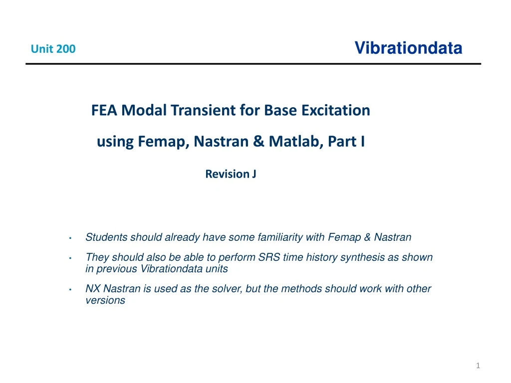
Unit 200 FEA Modal Transient for Base Excitation using Femap, Nastran & Matlab, Part I Revision J Students should already have some familiarity with Femap & Nastran They should also be able to perform SRS time history synthesis as shown in previous Vibrationdata units NX Nastran is used as the solver, but the methods should work with other versions
Introduction • Shock and vibration analysis can be performed either in the frequency or time domain • The time domain method requires more computation time but is much better suited for transient and nonstationary excitation • Modal transient analysis for base acceleration excitation is considered in this report • There are two methods for applying the acceleration as shown on the next page • The indirect seismic mass method is the subject for this presentation • The direct enforced acceleration method will be covered in a future presentation • Transient excitation using direct integration will also be covered in future units • The following software steps must be followed carefully, otherwise errors will result
Acceleration Excitation Methods Assume a rectangular plate mounted via posts at each corner F Rigid links • Directly enforce acceleration at corners • For uniform base excitation: • Mount plate to heavy seismic mass via rigid links • Apply force to yield desired acceleration at plate corners 3
Procedure, part I • Femap, NX Nastran and the Vibrationdata Matlab GUI package are all used in this analysis • The GUI package can be downloaded from: https://vibrationdata.wordpress.com/ • The first step is to load a library time history into Matlab using the GUI as shown in the following slides • The synthesized time history array name is: srs2000G_Accel • The time history is shown to satisfy an SRS specification • Its corresponding velocity and displacement time histories are stable and each has a net value of zero • The time history is then converted into a Nastran file using the GUI • The Nastran file is exported in ASCII text format as: srs2000G_accel.nas
Matlab: Vibrationdata GUI Type in Matlab Command Window: >> vibrationdata
Synthesized array name: srs2000G_accel • Units: time(sec) & accel(G) • The sample rate is 100K samples/sec which is 10 x the highest SRS natural frequency • The time histories is composed of a series of damped sinusoids which have been reconstructed in terms of wavelet
The synthesized time history satisfies the SRS specification within tolerance bands • Most pyrotechnic SRS specifications begin at 100 Hz • A good practice is to extrapolate the specification down to 10 Hz because the structure may have some lower modal frequencies
Matlab: Time History Set • Maintaining stable velocity & displacement are good engineering practice • Otherwise relative displacement error may occur due to significant digit effects if the displacement has a “ski slope” effect
Matlab: Vibrationdata GUI, Export • The 386 scale factor is used to convert the unit from G to in/sec^2 • Scale by 9.81 for conversion from G to m/sec^2 • The time history is exported as: srs2000G_accel.nas
Procedure, part II • Students should already have some experience constructing finite element models in Femap • Flat square plate 12 x 12 x 0.25 inch (0.305 x 0.305 x 0.00635 meters) • Define plate on XY plane so that Z-axis is perpendicular to the plate • Material: aluminum 6061-T651 • Use plate elements (quad4) • Each element is square with 0.25 x 0.25 inch (0.00635 x 0.00635 meters ) • 48 elements & 49 nodes per edge • Check for coincident nodes & merge accordingly • Renumber nodes beginning with 1 • Constrain all corner nodes for no TX, TY or TZ translation
Femap: Plate Nodes, Elements & Corner Constraints • The diagonal lines are drawn to identify the center point • Node 1201 is at the center in this model
Procedure, part III • Set up normal modes analysis in Femap • Solve for first 150 eigenvalues • Select Print & PostProcess • Save model as: square_plate_normal_modes.modfem (or pick your own name) • Students who have Femap with Nastran bundled together can do the analysis directly • Otherwise export analysis file as: square_plate_normal_modes.bdf (or whatever) • Run Nastran solver for: square_plate_normal_modes.bdf • Import square_plate_normal_modes.f06 into Femap to view mode shapes • View > Select > Deform • Optional: view the f06 file in Notepad++ application https://notepad-plus-plus.org/
Nodepad++: View f06 File • T3 is motion in the Z-axis • The set composed of modes 1, 6, 12 & 19 accounts for 98.9% of the T3 total mass
Femap: Mode Shape 1 • The fundamental mode at 117.6 Hz has 93.3% of the total modal mass in the T3 axis • The plate appears to behave almost as a single-degree-of-freedom system • But higher modes make a very significant contribution to the overall shock response
Femap: Mode Shape 6 • The sixth mode at 723 Hz has 3.6% of the total modal mass in the T3 axis
Femap: Mode Shape 12 • The twelfth mode at 1502 Hz has 1.6% of the total modal mass in the T3 axis
Femap: Mode Shape 19 • The 19th mode at 2266 Hz has only 0.3% of the total modal mass in the T3 axis • But it has the highest contribution to the T3 peak acceleration response at the center node to the input shock
Hand Calculation Check • Reference: Steinberg, Vibration Analysis for Electronic Equipment • The fundamental frequency fn for a flat square plate is
Hand Calculation Check (cont) • Aluminum mass per volume = 0.1 lbm/in^3 = 0.00025904 lbf sec^2/in^4 • Plate mass per area: ρ = (0.00025904 lbf sec^2/in^4)(0.25 in)= 6.476e-05 lbf sec^2/in^3 • Plate stiffness factor: D = (1.0e+07 lbf/in^2)(0.25 in)^3/(12(1-0.3^2)) = 1.431e+04 lbf in • Fundamental frequency: • fn = (1.13/ (12 in )^2)sqrt(1.431e+04 lbf in / 6.476e-05 lbf sec^2/in^3 ) • fn = 116.6 Hz • Hand calculation has very good agreement with FEA result 117.6 Hz • Next post-process f06 file in Matlab GUI
Matlab: Modal Density, One-third Octave Format • This plot could be useful for Statistical Energy Analysis (SEA)
Matlab: Modal Effective Mass Fractions • T3 is the out-of-plane bending axis • The dynamic analysis will be performed for the first twenty modes based on this table • Some consideration is also given to the maximum SRS frequency and the sample rate
Matlab: Node 1201 Eigenvectors Extract Eigenvector 1 node T1 T2 T3 R1 R2 R3 1201 7.394e-18 -1.256e-19 13.98 7.813e-12 4.043e-12 0 Extract Eigenvector 6 node T1 T2 T3 R1 R2 R3 1201 5.028e-15 -1.428e-16 -22.28 -2.212e-12 1.172e-12 0 Extract Eigenvector 12 node T1 T2 T3 R1 R2 R3 1201 -8.278e-13 -7.012e-13 2.499 6.68e-13 2.427e-12 0 Extract Eigenvector 19 node T1 T2 T3 R1 R2 R3 1201 -1.219e-12 -1.024e-12 -32.22 1.791e-12 -4.14e-13 0
Matlab: Node 1201 Parameters for T3 • The Participation Factors & Eigenvectors are shown as absolute values • The Eigenvectors are mass-normalized • The Eigenvectors are the only parameter in the table which depends on location • Modes 1, 6, 12 & 19 account for 98.9% of the total mass
Procedure, part IV • Prepare Femap model for modal transient analysis • Delete output set from normal modes analysis • Also: delete > model > functions • Set up damping function • Import time history: srs2000G_accel.nas • Edit corner node constraints • Add seismic mass to model • Set up dynamic analysis to apply acceleration time history to model • Femap will convert the acceleration time history to a force time history • Add some constraints
Femap: Q Damping • Customize the damping table according to your analysis problem need • Damping can vary with frequency • Q=10 is equivalent to 5% viscous modal damping
Femap: Import Nastran Acceleration Time History srs2000G_accel.nas
Femap: View Acceleration Time History • Modify > edit > function • NASTRAN TABLED2 is the function for srs2000G_accel.nas
Femap: Acceleration Time History • The X-axis is Time (sec) • The Y-axis is Acceleration (in/sec^2)
Femap: Constraints • Edit corner node constraints so that only TX & TY are fixed
Femap: Added Points and Node Node 2402 • Copy center point twice at -3 inch increments in the Z-axis • Place node on point at middle point
Femap: Configure Rigid Element, RBE2 • Dependent DOF is TZ • Dependent Nodes are the corner nodes • Node 2402 is the independent Node, -3 inch from plate’s center node in Z-axis
Femap: Plate with Rigid Element Rigid Link Node 2402