Download
1 / 61
620 likes | 766 Views
Gene Expression Analysis and Modeling. Guillaume Bourque Centre de Recherches Mathématiques Université de Montréal August 2003. http://www.sri.com/pharmdisc/cancer_biology/laderoute.html. DNA Microarrays. Experiment design Noise reduction Normalization … Data analysis. Outline.

E N D
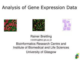
Gene Expression Analysis and Modeling Guillaume Bourque Centre de Recherches Mathématiques Université de Montréal August 2003
http://www.sri.com/pharmdisc/cancer_biology/laderoute.html DNA Microarrays • Experiment design • Noise reduction • Normalization • … • Data analysis Guillaume Bourque, CRM Summer School
Outline • Microarray data analysis techniques • Clustering: hierarchical and k-means • SVD and PCA • SVM – Support Vector Machines • Gene network modeling • Boolean networks • Bayesian models • Differential equations Guillaume Bourque, CRM Summer School
Outline • Microarray data analysis techniques • Clustering: hierarchical and k-means • SVD and PCA • SVM – Support Vector Machines • Gene network modeling • Boolean networks • Bayesian models • Differential equations Guillaume Bourque, CRM Summer School
Gene Expression Data Guillaume Bourque, CRM Summer School
gi = Transcriptional response of the ith gene aj = Expression profile of the jth assay Gene Expression Matrix Given an experiment with m genes and n assays we produce a matrix X where: xij= expression level of the ith gene in the jth assay. Guillaume Bourque, CRM Summer School
Goals of Clustering • Clustering genes: • Classify genes by their transcriptional response and get an idea of how groups of genes are regulated. • Potentially infer gene functions of unknown genes. • Clustering assays: • Classify diseased versus normal samples by their expression profile. • Track the expression levels at different stages in the cell. • Study the impact of external stimuli. Guillaume Bourque, CRM Summer School
similarity matrix cluster genes based on similarity m genes m genes Clustering Genes X m genes n assays Guillaume Bourque, CRM Summer School
Clustering Steps • Choose a similarity metric to compare the transcriptional response or the expression profiles: • Pearson Correlation • Spearman Correlation • Euclidean Distance • … • Choose a clustering algorithm: • Hierarchical • K-means • … Guillaume Bourque, CRM Summer School
Similarity Metric • Choice of the best metric depends on the normalization procedure. • Must be cautious of potential pitfalls. • Correlations:Correlation coefficients are values from –1 to 1, with 1 indicating a similar behavior, –1 indicating an opposite behavior and 0 indicating no direct relation. • Euclidean distance: Guillaume Bourque, CRM Summer School
g1 g4 Hierarchical Clustering • Find largest value is similarity matrix. • Join clusters together. • Recompute matrix and iterate. Guillaume Bourque, CRM Summer School
g2 g3 g1 g4 Hierarchical Clustering • Find largest value is similarity matrix. • Join clusters together. • Recompute matrix and iterate. Guillaume Bourque, CRM Summer School
g5 g2 g3 g1 g4 Hierarchical Clustering • Find largest value is similarity matrix. • Join clusters together. • Recompute similarity matrix and iterate. Guillaume Bourque, CRM Summer School
Cluster Joining • One of the issue with hierarchical clustering is how to recompute the similarity matrix after joining clusters. Here are 3 common solutions that define different types of hierarchical clustering: • Single-link: minimum distance between any member of one cluster to any member of the other cluster. • Complete-link: maximum distance between any member of one cluster to any member of the other cluster. • Average-link: average distance between any member of one cluster to any member of the other cluster. Guillaume Bourque, CRM Summer School
2 clusters ? 3 clusters ? g5 g2 g3 g1 g4 Interpreting the Results Guillaume Bourque, CRM Summer School
Clustering Example Eisen et al. (1998), PNAS, 95(25): 14863-14868 Guillaume Bourque, CRM Summer School
K-means Clustering k = 3 • Expression profiles are displayed in n dimensional space. • First cluster center is picked at random between all data points. • Other cluster centers are picked as far as possible from previous clusters centers. Guillaume Bourque, CRM Summer School
K-means Clustering k = 3 • Associate each data point to the closest cluster center. • Recompute cluster centers based on new clusters. Guillaume Bourque, CRM Summer School
K-means Clustering k = 3 • Associate each data point to the closest cluster center. • Recompute cluster centers based on new clusters. • Iterate until the clusters remain unchanged. Guillaume Bourque, CRM Summer School
K-means Clustering k = 3 • Associate each data point to the closest cluster center. • Recompute cluster centers based on new clusters. • Iterate until the clusters remain unchanged. Guillaume Bourque, CRM Summer School
K-means Clustering k = 3 • Associate each data point to the closest cluster center. • Recompute cluster centers based on new clusters. • Iterate until the clusters remain unchanged. Guillaume Bourque, CRM Summer School
vk= eigengene sk= singular value uk= eigenassay Singular Value Decomposition Xm x n = Um x n Sn x n V Tn x n (n m) = gene expression matrix Guillaume Bourque, CRM Summer School
Singular Value Matrix Sn x n = = Singular values are organized from largest to smallest: s1 s2 … sk … sn. Guillaume Bourque, CRM Summer School
Why SVD? • SVD extracts fromthe gene expression matrix: • n eigenassays • m eigengenes • n singular values • We can represent the transcriptional response of each gene as a linear combination of the eigengenes. • We can represent the expression profile of each assay as a linear combination of the eigenassays. • Allows for dimensionality reduction and for the identification of important components. Guillaume Bourque, CRM Summer School
SVD and PCA • There is a direct correspondence between SVD and PCA (Principal Component Analysis) when calculated on covariance matrices. • If we normalize X so that it’s columns have a 0 mean. We get that the eigengenes are the principal components of the transcriptional responses. • If we normalize X so that it’s rows have a 0 mean. We get that the eigenassays are the principal components of the expression profiles. • In both cases, we get that the square of the singular values are proportional to the variance of the principal components. Guillaume Bourque, CRM Summer School
U U S V T V T X(r) is the closest rank r approximation of X 0 0 0 SVD Special Property X = S(r) X(r)= where r is the number of non-null rows Guillaume Bourque, CRM Summer School
Applications of SVD • Detects redundancies and allows for the representation of the data with the minimal set of essential features (components). These features can themselves represent signals (e.g. cell-cyle). • Data visualization. SVD can identify subspaces that capture most of the variance in the data which allows for the visualization of high-dimensional data in 1, 2 or 3-dimensional subspace. • Signal extraction in noisy data. Guillaume Bourque, CRM Summer School
Essential Features Alteret al. (2000), PNAS, 97(18): 10101-10106 Guillaume Bourque, CRM Summer School
Data Visualization Yeung and Ruzzo. (2001), Bioinformatics, 17(9): 763-774 Guillaume Bourque, CRM Summer School
Support Vector Machines (SVM) • Instead of trying to identify clusters directly in the data, we assume the genes are already pre-clustered into different classes. The goal is the find a model that best predicts these classes. • We need to find the hyperplane that best divide the data points. • We must do so while minimize the error rates of the predictions. Guillaume Bourque, CRM Summer School
References • Clustering • deRisi et al. (1997), Science, 278(5338): 680-686. • Eisen et al. (1998), PNAS, 95(25): 14863-14868. • SVD and PCA • Alteret al. (2000), PNAS, 97(18): 10101-10106. • Holter et al. (2000), PNAS, 97(15): 8409-8414. • Yeung and Ruzzo. (2001), Bioinformatics, 17(9): 763-774. • Wall et al. (2003), A Pratical Approach to Microarray Data Analysis, Chapter 5. • SVM • Brown et al. (2000), PNAS, 97(1), 262-267. Guillaume Bourque, CRM Summer School
Outline • Microarray data analysis techniques • Clustering: hierarchical and k-means • SVD and PCA • SVM – Support Vector Machines • Gene network modeling • Boolean networks • Bayesian models • Differential equations Guillaume Bourque, CRM Summer School
_ x1 _ + ? _ x2 x3 + + _ x4 _ Gene network Problem Time series Guillaume Bourque, CRM Summer School
Boolean Networks • Genes are assumed to be ON or OFF. • At any given time, combining the gene states gives a gene activity pattern (GAP). • Given a GAP at time t, a deterministic function (a set of logical rules) provides the GAP at time t +1. • GAPs can be classified into attractor and transient states. Guillaume Bourque, CRM Summer School
transient attractors Boolean Network Example x1 x2 x3 t x1 x2 x3 t+1 or nor nand Guillaume Bourque, CRM Summer School
State Space Picture generated using the program DDLab. Wuensche,A., (1998), Proceedings of Complex Systems '98 . Guillaume Bourque, CRM Summer School
AND NAND NOT Boolean Network Example I. Shmulevich et al., Bioinformatics (2002), 18 (2): 261-274 Guillaume Bourque, CRM Summer School
Issues with Boolean Networks • Gene trajectories are continuous and modeling them as ON/OFF might be inadequate. • A deterministic set of logical rules forces a very stringent model. • It doesn’t allow for external input. • Very susceptible to noise. • Probability Boolean Networks aims at fixing some of these issues by combining multiple sets of rules (related to Bayesian Networks). Guillaume Bourque, CRM Summer School
Threshold(s) ON OFF Guillaume Bourque, CRM Summer School
Bayesian Networks • A gene regulatory network is represented by directed acyclic graph: • Vertices correspond to genes. • Edges correspond to direct influence or interaction. • For each gene xi, a conditional distribution p(xi | ancestors(xi) ) is defined. • The graph and the conditional distributions, uniquely specify the joint probability distribution. Guillaume Bourque, CRM Summer School
x1 x2 x4 x3 x5 Bayesian Network Example Conditional distributions: p(x1), p(x2), p(x3| x2), p(x4| x1,x2), p(x5| x4) p(X) = p(x1) p(x2| x1) p(x3| x1,x2) p(x4| x1,x2, x3) p(x5| x1,x2, x3,x4) p(X) = p(x1) p(x2) p(x3| x2) p(x4| x1,x2) p(x5| x4) Guillaume Bourque, CRM Summer School
Learning Bayesian Models • Using gene expression data, the goal is to find the bayesian network that best matches the data. • Recovering optimal conditional probability distributions when the graph is known is “easy”. • Recovering the structure of the graph is NP-hard. • But, good statistics are available: • What is the likelihood of a specific assignment? • What is the distribution of xi given xj? • … Guillaume Bourque, CRM Summer School
Issues with Bayesian Models • Computationally intensive. • Requires lots of data. • Does not allow for feedback loops which are known to play an important role in biological networks. • Does not make use of the temporal aspect of the data. • Dynamical Bayesian Networks aim at solving some of these issues but they require even more data. Guillaume Bourque, CRM Summer School
Differential Equations • Typically uses linear differential equations to model the gene trajectories:dxi(t) / dt = a0 + ai,1 x1(t)+ ai,2 x2(t)+ … + ai,n xn(t) • Several reasons for that choice: • lower number of parameters implies that we are less likely to over fit the data • sufficient to model complex interactions between the genes Guillaume Bourque, CRM Summer School
_ x1 _ + _ x2 x3 + + _ x4 _ Small Network Example dx1(t) / dt = 0.491 - 0.248 x1(t) dx2(t) / dt = -0.473 x3(t) + 0.374 x4(t) dx3(t) / dt = -0.427 + 0.376 x1(t) - 0.241 x3(t) dx4(t) / dt = 0.435 x1(t) - 0.315 x3(t) - 0.437 x4(t) Guillaume Bourque, CRM Summer School
Small Network Example _ x1 _ + _ x2 x3 + + _ x4 oneinteraction coefficient _ dx1(t) / dt = 0.491 - 0.248 x1(t) dx2(t) / dt = -0.473 x3(t) + 0.374 x4(t) dx3(t) / dt = -0.427 + 0.376 x1(t) - 0.241 x3(t) dx4(t) / dt = 0.435 x1(t) - 0.315 x3(t) - 0.437 x4(t) Guillaume Bourque, CRM Summer School
_ x1 _ + _ x2 x3 + + _ x4 _ Small Network Example constant coefficients dx1(t) / dt = 0.491 - 0.248 x1(t) dx2(t) / dt = -0.473 x3(t) + 0.374 x4(t) dx3(t) / dt = -0.427 + 0.376 x1(t) - 0.241 x3(t) dx4(t) / dt = 0.435 x1(t) - 0.315 x3(t) - 0.437 x4(t) Guillaume Bourque, CRM Summer School
Problem Revisited Given the time-series data, can we find the interactions coefficients? Guillaume Bourque, CRM Summer School
Issues with Differential Equations • Even under the simplest linear model, there are m(m+1) unknown parameters to estimate: • m(m-1) directional effects • m self effects • m constant effects • Number of data points is mn and we typically have that n << m (few time-points). • To avoid over fitting, extra constraints must be incorporated into the model such as: • Smoothness of the equations • Sparseness of the network (few non-null interaction coefficients) Guillaume Bourque, CRM Summer School
Algorithm for Network Inference • To recover the interaction coefficients, we use stepwise multiple linear regression. • Why? • This procedure only finds coefficient that significantly improve the fit in the regression. Hence it limits the number of non-zero coefficients (i.e. it finds sparse networks) a feature we were seeking. • It is highly flexible and provides p-value scores which can be interpreted easily. Guillaume Bourque, CRM Summer School