Download
1 / 19
250 likes | 566 Views
Bootstrap. Bootstrapping applied to t-tests. Problems with t . Wilcox notes that when we sample from a non-normal population, assuming normality of the sampling distribution maybe optimistic without large samples

E N D
Bootstrap Bootstrapping applied to t-tests
Problems with t • Wilcox notes that when we sample from a non-normal population, assuming normality of the sampling distribution maybe optimistic without large samples • Furthermore, outliers have an influence on both the mean and sd used to calculate t • Actually has a larger effect on variance, increasing type II error due to std error increasing more so than the mean • This is not to say we throw the t-distribution out the window • If we meet our assumptions and have ‘pretty’ data, it is appropriate • However, if we cannot meet the normality assumption we may have to try a different approach • E.g. bootstrapping
More issues with the t-test • In the two-sample case we have an additional assumption (along with normality and independent observations) • We assume that there are equal variances in the groups • Recall our homoscedasticity discussion • Often this assumption is untenable, and the results, like other violations result in using calculated probabilities that are inaccurate • Can use a correction, e.g. Welch’s t
More issues with the t-test • It is one thing to say that they are unequal, but what might that mean? • Consider a control and treatment group, treatment group variance is significantly greater • While we can do a correction, the unequal variances may suggest that those in the treatment group vary widely in how they respond to the treatment • Another reason for heterogeneity of variance may be related to an unreliable measure being used • No version of the t-test takes either into consideration • Other techniques, assuming enough information has been gathered, may be more appropriate (e.g. hierarchical), and more reliable measures may be attainable *Note that, if those in the treatment are truly more variable, a more reliable measure would actually detect this more so (i.e. more reliability would lead to a less powerful test). We will consider this more later.
The good and the bad regarding t-tests • The good • If assumptions are met, t-test is fine • When assumptions aren’t met, t-test may still be robust with regard to type I error in some situations • With equal n and normal populations HoV violations won’t increase type I much • With non-normal distributions with equal variances, type I error rate is maintained also • The bad • Even small departures from the assumptions result in power taking a noticeable hit (type II error is not maintained) • t-statistic, CIs will be biased
Bootstrap • Recall the notion of a sampling distribution • We never have the population available in practice, so we take a sample (one of an infinite amount of possible ones) • The sampling distribution is a theoretical distribution whose shape we assume
Bootstrap • The basic idea involves sampling with replacement from the sample data (essentially treating it as the population) to produce random samples of size n • We create an empirical sampling distribution • Each of these samples provides an estimate of the parameter of interest • Repeating the sampling a large number of times provides information on the variability of the estimator
Bootstrap • Hypothetical situation: • If we cannot assume normality, how would we go about getting a confidence interval? • Wilcox suggests that assuming normality via the central limit theorem doesn’t hold for small samples, and sometimes could require as much as 200 to maintain type I error if the population is not normally distributed • If we do not maintain type I error, confidence intervals and inferences based on them will be suspect • How might you get a confidence interval for something besides a mean? • Solution: • Resample (with replacement) from our own data based on its distribution • Treat our sample as a population distribution and take random samples from it
The percentile bootstrap • We will start by considering a mean • We can bootstrap many sample means based on the original data • One method would be to simply create this distribution of means, and note the percentiles associated with certain values
The percentile bootstrap • Here are some values (from Wilcox text), mental health ratings of college students • Mean = 18.6 • Bootstrap mean (k =1000) = 18.52 • The bootstrapped 95% CI is • 13.85, 23.10 • Assuming normality • 13.39, 23.81 • Different coverage (non-symmetric for bootstrap), and the classical approach is noticeably wider 2,4,6,6,7,11,13,13,14,15,19,23,24,27,28,28,28,30,31,43
The percentile t bootstrap • Another approach would be to create an empirical t distribution • Recall the formula for a one-sample t • For our purposes here, we will calculate a t, 1000 times, as follows. With each mean and standard deviation of 1 of those 1000 samples, calculate
The percentile t bootstrap • This would give us a t distribution with 1000 t scores • What we would now do for a confidence interval is find the exact t corresponding to the appropriate quantiles (e.g. .025,.975), and use those to calculate a CI using the original sample statistics
Confidence Intervals • So what we have done is, instead of assuming some sampling distribution of a particular shape and size, we’ve created it ourselves and derived our interval estimate from it • Simulations have shown that this approach is preferable for maintaining type I error with larger samples in which the normality assumption may be untenable.
Independent Groups • Comparing independent groups • Step 1 compute the bootstrap mean and bootstrap sd as before, but for each group • Each time you do so, calculate T* • This again creates your own t distribution.
Hypothesis Testing • Use the quantile points corresponding to your confidence level in computing your confidence interval on the difference between means, rather than the tcv from typical distributions • Note however that your T* will not be the same for the upper and lower bounds • Unless your bootstrap distribution was perfectly symmetrical • Not likely to happen, so…
Hypothesis Testing • One can obtain ‘symmetric’ intervals • Instead of using the value obtained in the numerator (mean-mu) or (diff b/t means – mu1-mu2), use its absolute value • Then apply the standard + formula • This may in fact be the best approach for most situations
Extension • We can incorporate robust measures of location rather than means • Eg. Trimmed means • With a program like R it is very easy to do both bootstrapping and with robust measures using Wilcox’s libraries • http://psychology.usc.edu/faculty_homepage.php?id=43 • Put the Rallfun files (most recent) in your version 2.x main folder and ‘source’ them, then you’re ready to start using such functionality • E.g. source(“Rallfunv1.v5”) • Example code on last slide • The general approach can also be extended to more than 2 groups, correlation, and regression
So why use? • Accuracy and control of type I error rate • As opposed to just assuming that it’ll be ok • Most of the problems associated with both accuracy and maintenance of type I error rate are reduced using bootstrap methods compared to Student’s t • Wilcox goes further to suggest that there may be in fact very few situations, if any, in which the traditional approach offers any advantage over the bootstrap approach • The problem of outliers and the basic statistical properties of means and variances as remain however
Example independent samples t-test in R • source("Rallfunv1.v5") • source("Rallfunv2.v5") • y=c(1,1,2,2,3,3,4,4,5,7,9) • z=c(1,3,2,3,4,4,5,5,7,10,22) • t.test(y,z, alpha=.05) • yuenbt(y,z,tr=.0,alpha=.05,nboot=600,side=T)