Efficient Strategies for Mesh Generation in Rapidly Evolving PDE Solutions

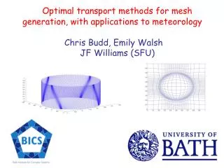
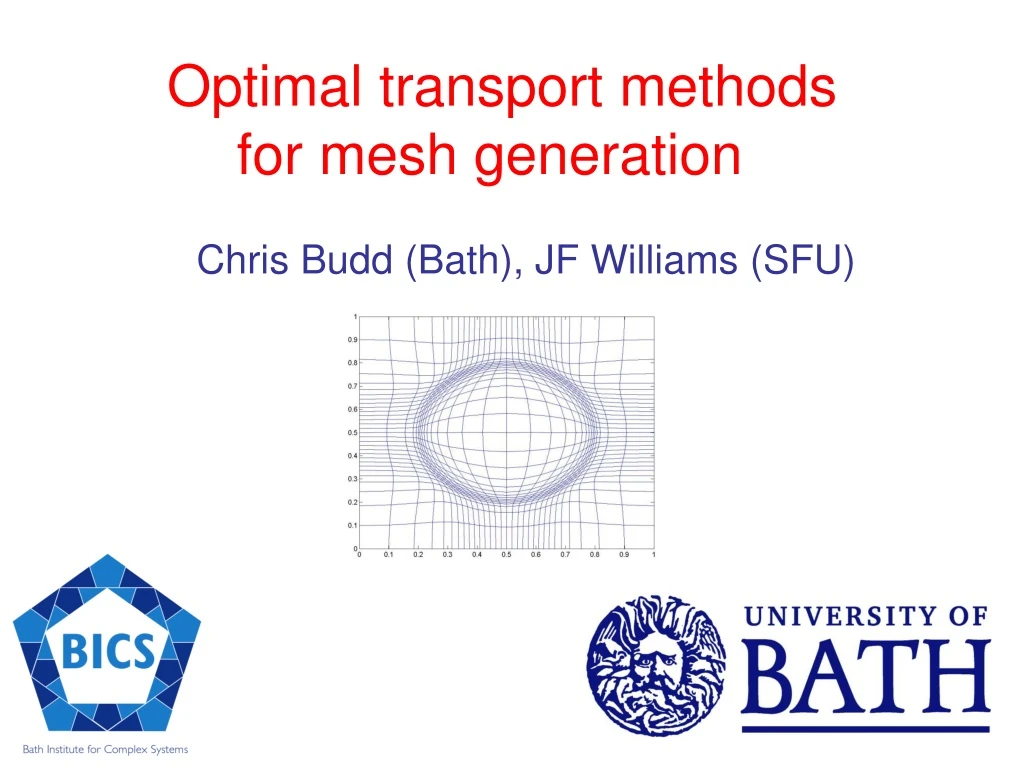
1. Optimal transport methods for mesh generation Chris Budd (Bath), JF Williams (SFU)

2. Have a PDE with a rapidly evolving solution u(x,t) How can we generate a mesh which effectively follows the solution structure? • h-refinement • p-refinement • r-refinement Also need some estimate of the solution/error structure which may be a-priori or a-posteriori Will describe an efficient n-dimensional r-refinement strategy using a-priori estimates

3. r-refinement Strategy for generating a mesh by mapping a uniform mesh from a computational domain into a physicaldomain F Need a strategy for computing the mesh mapping function F which is both simple and fast

4. Equidistribution: 2D Introduce a positive unit measureM(X,Y,t) in the physical domain which controls the mesh density A : set in computational domain F(A) : image set Equidistribute image with respect to the measure

5. JF: I wrote this talk using the assumption of unit measure for M as it simplifies the presentation. Of course we don’t need this in general

6. Differentiate: Basic, nonlinear, equidistribution mesh equation

7. Equidistribution in one-dimension This is a very well defined process Let computational and physical domains both be the unit interval [0,1]. Mesh function X(xi) X(0) = 0, X(1) = 1 Basic mesh equation: unique solution if M>0

8. Hard, and unecessary, to solve exactly! Various approaches to the solution … 1. Geometric conservation Solve for V

9. Some CJB notes on possible issues with GCL • Have to start with an equidistributed mesh • Have to know M_t • Have to calculate V then calculate X • Potential problems with mesh crossing • Generalises to higher dimensions

10. 2. Relaxation Evolve towards an equidistributed mesh (MMPDE5) or Mesh PDE [Russell] (MMPDE6) Very effective provided that the time-scales for the mesh evolution are smaller than those for the evolution of the underlying PDE: MOVCOL Code [Huang, Russell]

11. Implementation: Underlying PDE solution: Moving mesh: Approximate solution: Discretise Underlying PDE (in Lagrangian form) and Mesh PDE in thecomputational variable Solve the resulting ODEs

12. Back to two-dimensions Problem: in two-dimensions equidistribution does NOT uniquely define a mesh! All have the same area Need additional conditions to define the mesh Also want to avoid mesh tangling and long thin regions

13. Optimally transported meshes F Argue: A good mesh is one which is as close as possible to a uniform mesh

14. Monge-Kantorovich optimal transport problem Minimise Subject to Also used in image registration,meteorology

15. Intuitively a good approach Small I A = 2 A = 1 Larger I A = 2 Optimal transport helps to prevent small angles

16. Brenier’s polar factorisation theorem Key result which makes everything work!!!!! • Theorem: [Brenier] • There exists a unique optimally transported mesh • (b) For such a mesh the map F is the gradient of a convex function P : Scalar mesh potential Map F is a Legendre Transformation

17. Some corollaries of the Polar Factorisation Theorem Gradient map Irrotational mesh Convexity of P prevents mesh tangling

18. Some simple examples Uniform enlargement scale factor 1/M Linear map. A is symmetric positive definite Tensor product mesh

19. It follows immediately that Hence the mesh equidistribustion equation becomes (MA) Monge-Ampere equation: fully nonlinear elliptic PDE

20. Basic idea: Solve (MA) for P with appropriate (Neumann) boundary conditions Good news: Equation has a unique solution Bad news: Equation is very hard to solve Good news: We don’t need to solve it exactly! Use relaxation as in the MMPDE equations

21. Relaxation uses a combination of a rescaled version of MMPDE5 and MMPDE6 in 2D (PMA) Spatial smoothing (Invert operator using a spectral method) Ensures right-hand-side scales like Q in 2D to give global existence Averaged monitor Parabolic Monge-Ampere equation

22. Discretise and solve PMA in parallel with the Lagrangian form of the PDE (possibly using a temporal rescaling) Useful properties of PMA • Lemma 1: [Budd,Williams 2006] • If M(X,t) = M(X) then PMA admits the solution • (b) This solution is locally stable. Proof: Follows from the convexity of P which ensures that PMA behaves locally like the heat equation

23. Lemma 2: [Budd,Williams 2006] If M(X,t) is slowly varying then the grid given by PMA is epsilon close to that given by solving the Monge Ampere equation. Lemma 3: [Budd,Williams 2006] The mapping is 1-1 and convex for all times

24. Additional issues for CJB and JFW • If M is slowly varying then Q stays epsilon close to the solution of the Monge-Ampere equation • Need rigorous proof that Q remains convex and of global convergence and a maximum principle • When we solve in a rectangular domain then there is a mild loss of regularity in the corners. • There is also an boundary orthogonality of the grid in the physical domain. This is both good and bad

25. Lemma 4: [Budd,Williams 2005] If there is a natural length scale L(t) then for careful choices of M the PMA inherits this scaling and admits solutions of the form Extremely useful property when working with PDEs which have natural scaling laws eg.

26. Examples of applications 1. Prescribe M(X,t) and solve PMA

27. 2. Solve in parallel with the PDE 10 10^5 Solution: Y X Mesh:

28. Solution in the computational domain 10^5

29. Conclusions • Optimal transport is a natural way to determine meshes in dimensions greater than one • It can be implemented using a relaxation process by using the PMA algorithm • Method works well for a variety of problems, and there are rigorous estimates about its behaviour • Still lots of work to be done eg. Finding efficient ways to couple PMA to the underlying PDE