Download
1 / 16
160 likes | 850 Views
Re-Order Point Problems Set 3: Advanced. Problem 7.2.

E N D
Problem 7.2 Weekly demand for DVD-Rs at a retailer is normally distributed with a mean of 1,000 boxes and a standard deviation of 150. Currently, the store places orders via paper that is faxed to the supplier. Assume 50 working weeks in a year. Lead time for replenishment of an order is 4 weeks. Fixed cost (ordering and transportation) per order is $100. Each box of DVD-Rs costs $1. Annual holding cost is 25% of average inventory value. The retailer currently orders 20,000 DVD-Rs when stock on hand reaches 4,200. a.1) How long, on average, does a box of DVD-R spend in the store? Isafety= ROP – LTD LTD = L×R = 4×1000 = 4000 Isafety= 4200 -4000 = 200 Icycle =Q/2 = 20000/2 Average inventory = Icycle + Isafety I = Average Inventory = 20000/2 + 200= 10200 I = RT 10200 = 1000T = 10.2 weeks R/week = N(1000,150) L = 2 week Q = 20,000 ROP = 4,200 50 weeks /yr Ave. R /year = 50,000 S =100 C = 1 Carrying cost = 25% of purchasing cost. H=0.25C = $0.25
=6325 Problem 7.2a a.2) What is the annual ordering and holding cost. Number of orders R/Q R/Q = 50,000/20,000 = 2.5 Ordering cost = 100(2.5) = 250 Annual holding cost = 0.25% ×1 ×10200 =2550 Total inventory system cost excluding purchasing = 250+2550 = 2800. b.1) Assuming that the retailer wants the probability of stocking out in a cycle to be no more than 5%, recommend an optimal inventory policy (a policy regarding order quantity and safety stock).
Problem7.2b Z(95%) = 1.65 Z(95%) = 1.65 Isafety = zσLTD =1.65(300) = 495 ROP = 4000+195 = 4495 Optimal Policy: Order 6325 whenever inventory on hand is 4495 b.2) Under your recommended policy, how long, on average, would a box of DVD-Rs spend in the store? Average inventory = 6325/2 + 495 Average inventory = 3658 I = RT 3658 = 1000T T = 3.66 weeks
Problem 7.2b-c c) Reduce lead time form 4 to 1. What is the impact on cost and flow time? Safety stock reduces from 495 to 247.5 247.5 units reduction That is 0.25(247.5) = $62 saving Average inventory = Icycle + Isafey = Q/2 + Isafety Average Inventory = I = (6,325/2) + 247.5 = 3,410. Average time in store I = RT 3410 = 1000T T = 3.41 weeks
=24980 Problem 7.3 Home and Garden (HG) chain of superstores imports decorative planters from Italy. Weekly demand for planters averages 1,500 with a standard deviation of 800. Each planter costs $10. HG incurs a holding cost of 25% per year to carry inventory. HG has an opportunity to set up a superstore in the Phoenix region. Each order shipped from Italy incurs a fixed transportation and delivery cost of $10,000. Consider 52 weeks in the year. R/week = N(1500,800) C = 10 h = 0.25 H =0.25(10) = 2.5 52 weeks /yr R = 78000/yr S =10000 L = 4 weeks SL = 90% a) Determine the optimal order quantity (EOQ). b) If the delivery lead time is 4 weeks and HG wants to provide a cycle service level of 90%, how much safety stock should it carry?
Problem 7.3c- Rough Computation c) Reduce L from 4 to 1, Increase C by 0.2 per unit. Yes or no? c.1) Rough computations. Purchasing cost increase 0.2(78000) = 15600 Safety stock decrease from 2048 to 1024 1024 units reduction Safety stock cost saving = 2.5(1024) = 2560 15600-2560 = 13040 increase in cost
Problem 7.3c – Detailed Computation c.1) Detailed computations. R/week = N(1500,800) C = 10 + 0.2 H = .25(10+.2) = 2.55 52 weeks /yr R = 78000 S =10000 L = 4 weeks SL = 90% For the original case of C = 10 and H =2.5 +HIs +CR Change in C Change in H. Not only purchasing cost changes But also cost of EOQ and Is Changes Reduce L from 4 to 1 Purchasing cost increase = 0.2(78000) = 15600 Safety stock reduces from 2048@2.5 to 1024@2.55 Safety stock cost saving = 2.5(2048)-2.55(1024) = 2509
Problem 7.3c – Detailed Computation Total inventory cost (ordering + carrying) will also increase R/week = N(1500,800) C = 10 + 0.2 H = .25(10+.2) = 2.55 52 weeks /yr R = 78000 S =10000 L = 4 weeks SL = 90% Total inventory cost (ordering + carrying) increase = 0.00995*62450 = 621 Total impact = +621+15600-2509 = 13712
Problem 7.8 – Centralization vs. Decentralization # of warehouses = 4 R/week at each warehouse = 10,000. 50 weeks per year R = N(10,000, 2,000) H=0.25(10) = 2.5 /yr S = 1000 L = 1 week σLTD = 2,000 SL = 0.95 =20000 z(0.95) = 1.65, σLTD = 2,000 Is = 1.65 x 2,000 = 3,300. 1×10,000 + 3,300 = 13,300. ROP = LTD + Is = Average inventory at each warehouse : Each time we order Q=20000 Icycle = Q/2 = 20000/2=10000 Average Inventory = Ic =10000+ 3300 =13300 + Is Average Decentralized inventory in 4 warehouses = =4(13300) = 53200 Demand in in 4(10000) =40000/w Demand in in 4 warehouses = RT = I 40000T= 53200 T = 1.33 weeks
Problem 7.8 – Centralization vs. Decentralization We do not consider RC because it does not depend on the inventory policy. But you can always add it. Inventory system cost for one warehouse Inventory system cost for four warehouses = 4(58,250) Inventory system cost for four warehouses = 233,000
b. Centralized Policy R/week in each warehouse follows Normal distribution with mean of 10,000, and Standard deviation of 2,000 When combining all in a central warehouse Mean (central) = 4(10000) = 40000 =40000 Variance (central) = 4(variance at each warehouse) Variance at each warehouse = (2000)2 = 4,000,000 Variance (central) = 4(4,000,000) = 16,000,000 Standard deviation (central) = 4,000 R (central) = Normal(40,000, 4000)
Centralized Policy The replenishment lead time (L) = 1week. Standard deviation of demand during lead time in the centralized system is: σLTD (all warehouses) = N σLTD(each warehouse) σLTD (all warehouses) =4 (2000) = 4000 Safety stock at each store for 95% level of service Isafety (central) = 1.65 x 4,000 = 6,600. Average inventory in the centralized system I = Q/2 +Isafety I = Icycle +Isafety 40000/2 +6600 =26600 Average Centralized Inventory = 26600 Average Decentralized Inventory = 53200 Average time spend in inventory (C): RT =I 4000T = 26600 T = 0.67
Total Cost We do not consider RC because it does not depend on the inventory policy. But you can always add it. Inventory system cost for four warehouse in centralized system Inventory system cost for four warehouses in decentralized system
Problem 7.9 – Centralization vs Decentralization EOQ at each warehouse # of warehouses = 4 Year = 50 weeks Rat each warehouse = 4,000/wk or 200,000 yr C= 200 H=0.2(200) = 40 /yr S = 900 (Decentralized) S = 1800 (Centralized) =3000 b) Average flow time T = 0.375 week RT=I 4000T=3000/2 c) Inventory system cost Inventory system cost for any Q is Inventory system cost for optimal EOQ is The total cost for all CC outlets for decentralized policy is
7.9 part (c) For centralized system RC = 4R and SC = 2S