Download
1 / 79
800 likes | 1.55k Views
Statistical Learning. Dong Liu Dept. EEIS, USTC. Chapter 1. Linear Regression. From one to two Regularization Basis functions Bias-variance decomposition Different regularization forms Bayesian approach. A motivating example 1/2. What is the height of Mount Qomolangma ?

E N D
Statistical Learning Dong Liu Dept. EEIS, USTC
Chapter 1.Linear Regression • From one to two • Regularization • Basis functions • Bias-variance decomposition • Different regularization forms • Bayesian approach Chap 1. Linear Regression
A motivating example 1/2 • What is the height of Mount Qomolangma? • A piece of knowledge – one variable • How do we achieve this “knowledge” from data? • We have a series of measurements: • For example, we can use the (arithmetic) mean: def HeightOfQomolangma(): return 8848.0 def SLHeightOfQomolangma(data): return sum(data) / len(data) Chap 1. Linear Regression
A motivating example 2/2 • Or in this way hQomo = 0 def LearnHeightOfQomolangma(data): global hQomo hQomo = sum(data) / len(data) def UseHeightOfQomolangma(): global hQomo return hQomo Learning/Training Using/Testing Chap 1. Linear Regression
Why arithmetic mean? • Least squares • Solving the problem • Relative (local) minimum • Absolute (global) minimum • In statistical learning, we often formulate such optimization problems and try to solve them • How to formulate? • How to solve? Chap 1. Linear Regression
From the statistical perspective • The height of Qomolangma is a random variable , which obeys a specific probability distribution • For example, Gaussian (normal) distribution • The measurements are observations of the random variable, and are used to estimate the distribution • Assumption: independent and identical distribution (i.i.d.) Chap 1. Linear Regression
Maximum likelihood estimation • Likelihood function: as a function of • Overall likelihood function (recall iid): • We need to find a parameter that maximizes the overall likelihood: • And it reduces to least squares! Chap 1. Linear Regression
More is implied • We can also estimate other parameters, e.g. • We can use other estimators, like unbiased: • We can give range estimation rather than point estimation Chap 1. Linear Regression
Correlated variables • The height of Mount Qomolangma is correlated to the season • So what is the correlation between two variables? • Why not an affine function: Spring Summer Fall Winter def UseSeasonalHeight(x, a, b): return a*x+b Chap 1. Linear Regression
Least squares • We formulate the optimization problem as • And (fortunately) have the closed-form solution • Result ↗ • Seemingly not good, how to improve? Chap 1. Linear Regression
Variable (re)mapping • Previously we use • Now we use • Result ↗ def ErrorOfHeight(datax, datay, a, b): fity = UseSeasonalHeight(datax, a, b) error = datay - fity return sum(error**2) Season: 3.6146646254138832 Remapped season: 0.9404394822254982 Chap 1. Linear Regression
From the statistical perspective • We have two random variables • Height: a dependent, continuous variable • Season: an independent, discrete variable • The season’s probability distribution • The height’s probability distribution • The overall likelihood function: Chap 1. Linear Regression
History review Carl Friedrich Gauss (German, 1777-1855) Adrien-Marie Legendre (French, 1752-1833) Chap 1. Linear Regression
Notes • Correlation is not Causality, but inspires efforts to interpret • Remapped/Latent variables are important Chap 1. Linear Regression
Chapter 1.Linear Regression • From one to two • Regularization • Basis functions • Bias-variance decomposition • Different regularization forms • Bayesian approach Chap 1. Linear Regression
As we are not confident about our data • Height is correlated to season, but also correlated to other variables • Can we constrain the level of correlation between height and season? • So we want to constrain the slope parameter • We have two choices • Given a range of possible values of slope parameter, find the least squares • Minimize the least squares and the (e.g. square of) slope parameter simultaneously Chap 1. Linear Regression
Two optimization problems • Constraint form • Unconstrained form • Solution Reg 0: y = 1.184060 * x +8846.369904, error: 0.940439 Reg 1: y = 1.014908 * x +8846.708207, error: 1.112113 Reg 2: y = 0.888045 * x +8846.961934, error: 1.466188 Reg 3: y = 0.789373 * x +8847.159277, error: 1.875104 Reg 4: y = 0.710436 * x +8847.317152, error: 2.286357 Reg 5: y = 0.645851 * x +8847.446322, error: 2.678452 Reg 6: y = 0.592030 * x +8847.553964, error: 3.043435 Reg 7: y = 0.546489 * x +8847.645045, error: 3.379417 Reg 8: y = 0.507454 * x +8847.723115, error: 3.687209 Reg 9: y = 0.473624 * x +8847.790776, error: 3.968753 Reg 10: y = 0.444022 * x +8847.849978, error: 4.226370 Chap 1. Linear Regression
How to solve a constrained optimization problem? • Consider a general optimization problem • The basic idea is to construct an augmented objective function where and are Lagrange multipliers • Then consider the dual function • When , the dual function is a lower bound of the original problem Chap 1. Linear Regression
Duality • The dual problem • Weak duality (always true) • Strong duality (under some condition) • Considering differentiable functions, strong duality implies • For convex optimization, KKT condition implies strong duality KKT condition Chap 1. Linear Regression
Understanding the KKT condition: From the equivalence of constrained and unconstrained • Equation as constraint • Inequation as constraint Chap 1. Linear Regression
Understanding the KKT condition: From the geometrical perspective Example: • No constraint • With equality as constraint • With inequality as constraint Chap 1. Linear Regression
More about convex optimization 1/2 • Convex set • Convex function • A function that is defined on a convex set • Concave function: if its negative is convex • Affine function is both convex and concave • Convex optimization is to minimize a convex function (or maximize a concave function) over a convex set Chap 1. Linear Regression
More about convex optimization 2/2 • For a convex optimization problem, any local minimum is also global minimum • Proof: by reductio • For a convex optimization problem, if the function is strictly convex, then there is only one global minimum • Proof: the definition of convex function • The dual problem is convex optimization Chap 1. Linear Regression
What & Why is regularization? • What • A process of introducing additional information in order to solve an ill-posed problem • Why • Want to introduce additional information • Have difficulty in solving the ill-posed problem With regularization: Without regularization: Chap 1. Linear Regression
From the statistical perspective • The Bayes formula • Maximum a posterior (MAP) estimation (Bayesian estimation) • We need to specify a prior, e.g.: • Finally it reduce to the regularized least squares with Chap 1. Linear Regression
Bayesian interpretation of regularization • The prior is “additional information” • Many statisticians question this point • How much regularization depends on • How confident we are about the data • How confident we are about the prior Chap 1. Linear Regression
Chapter 1.Linear Regression • From one to two • Regularization • Basis functions • Bias-variance decomposition • Different regularization forms • Bayesian approach Chap 1. Linear Regression
Polynomial curve fitting • Basis functions • Weights • Another form: weights and bias Chap 1. Linear Regression
Basis functions Global vs. Local Polynomial Gaussian Other choices: Fourier basis (sinusoidal), wavelet, spline Sigmoid Chap 1. Linear Regression
Variable remapping • Using basis functions will remap the variable(s) in a non-linear manner • Change the dimensionality • To enable a simpler (linear) model Chap 1. Linear Regression
Maximum likelihood • Assume observations are from a deterministic function with additive Gaussian noise • Then • Given observed inputs and targets • The likelihood function is Chap 1. Linear Regression
Maximum likelihood and least squares • Maximizing is equivalent to minimizing which is known as sum of squared errors (SSE) Chap 1. Linear Regression
Maximum likelihood solution • Solution is The design matrix The pseudo-inverse Chap 1. Linear Regression
Geometrical interpretation • Let • And let the columns of be • They span a subspace • Then, is the orthogonal projection of on the subspace , so as to minimize the Euclidean distance Chap 1. Linear Regression
Regularized least squares • Construct the “joint” error function • Use SSE as data term, and quadratic regularization term (ridge regression): • The solution is Data term + Regularization term Chap 1. Linear Regression
Equivalent kernel • For a new input, the predicted output is • Predictions can be calculated directly from the equivalent kernel, without calculating the parameters Equivalent kernel Chap 1. Linear Regression
Equivalent kernel for Gaussian basis functions Chap 1. Linear Regression
Equivalent kernel for other basis functions Polynomial Sigmoidal Equivalent kernel is “local”: nearby points have more weights Chap 1. Linear Regression
Properties of equivalent kernel • Sums to 1 if is 0 • May have negative values • Can be seen as inner product Chap 1. Linear Regression
Chapter 1.Linear Regression • From one to two • Regularization • Basis functions • Bias-variance decomposition • Different regularization forms • Bayesian approach Chap 1. Linear Regression
Example Reproduced from PRML • Generate 100 data sets, each having 25 points • A sine functionplus Gaussian noise • Perform ridge regression on each data set with 24 Gaussian basis functions and different values of regularization weight Chap 1. Linear Regression
Simulation results 1/3 • High regularization, the variance is small but bias is large Fitted curve (shown 20 fits) The average curve after 100 fits Chap 1. Linear Regression
Simulation results 2/3 • Moderate regularization Fitted curve (shown 20 fits) The average curve after 100 fits Chap 1. Linear Regression
Simulation results 3/3 • Low regularization, the variance is large but bias is small Fitted curve (shown 20 fits) The average curve after 100 fits Chap 1. Linear Regression
Bias-variance decomposition • The second term is intrinsic “noise”, consider the first term • Suppose we have a dataset and we can calculate the parameter based on the dataset • Then we take expectation with respect to dataset • Finally we have: expected “loss” = (bias)2 + variance + noise Chap 1. Linear Regression
Bias-variance trade-off • Over-regularized modelwill have a high bias, while under-regularized modelwill have a high variance • How can we achieve the trade-off? • For example, by cross validation (will be discussed later) Chap 1. Linear Regression
Chapter 1.Linear Regression • From one to two • Regularization • Basis functions • Bias-variance decomposition • Different regularization forms • Bayesian approach Chap 1. Linear Regression
Other forms? • Least squares • Ridge regression • Norm regularized regression norm: Chap 1. Linear Regression
Different norms What about 0 and ∞? Chap 1. Linear Regression
Best subset selection • Define “norm” as • Best subset selection regression: • Also known as “sparse” • Unfortunately, this is NP-hard Chap 1. Linear Regression