Download
1 / 33
340 likes | 490 Views
Interpreting Hysteresis in Concentration/Discharge Models using a Mixing Approach. Richard P. Hooper and Beth Rudolph U.S. Geological Survey Northborough, Mass. Concentration/Discharge Models. Important in water-quality studies Loads/Output budgets Trend analysis Poorly posed statistically

E N D
Interpreting Hysteresis in Concentration/Discharge Models using a Mixing Approach Richard P. Hooper and Beth Rudolph U.S. Geological SurveyNorthborough, Mass.
Concentration/Discharge Models • Important in water-quality studies • Loads/Output budgets • Trend analysis • Poorly posed statistically • Residuals are not I.I.D. even after transformations • Event samples appear different from baseflow • Normally don’t account for hysteresis • Implications • Precision estimates questionable • Trend Analysis suspect
Mixing Models • Successful in many catchments • Often 3-component mixtures • Can capture hysteresis • Different mixing proportions on rising and falling limb • No direct way to link C/Q and mixing • Assume hydrology of components • Two-component mixtures can lead to hyperbolic and power-law models • No easy extension to 3 components
Evans and Davies [1998] • C/Q loop shape and direction implied concentration order of end members • Use a single “typical” hydrograph • Subsequent studies by Chanat et al. [in press] showed not one-to-one relation with moderate uncertainty
E&D Flow Components • Derive from DeWalle and Swistock’s ideas • Not independently measured solutions • Combined hydrologic processes and tracers • Surface Event Water • Precipitation directly on saturated zone near stream • Soil Water • Water converted from vadose zone (prior to event) • Groundwater • Assumed equivalent to baseflow
This Study • Examine end-member contributions for 28 storms (WY86-88; WY93-98) • Similar to E&D master hydrograph? • Patterns of contributions • Relate response to antecedent conditions and storm characteristics • Implications for concentration/discharge models
Hydrograph Separation Re-express Hydrograph Separation on Ternary Diagram
Panola Mountain Research Watershed • 41-ha catchment near Atlanta, GA • Perennial stream at outlet • Event sampling: WY86-88 and WY 93-98 • End Members: • Lower Groundwater (Site 325) • Upper Groundwater (Site 760 [WY86-88]; Site 803 [WY93-98]) • Vadose Water (Site 640)
End member definitions • Lower Groundwater (LGW)= E&D groundwater • Upper Groundwater (UGW) = E&D Soil water • Vadose Water (VW) = E&D Surface Event Water
End-member Mixing Analysis • Over-determined system (6 tracers when 3 are needed) • Determine 2-dimension mixing subspace using PCA • Project end-member median concentration into mixing subspace (time invariant em’s) • Calculate mixing proportions subject to non-negativity constraint
General EM Contribution Patterns • Storm begins along LGW/UGW axis and proceeds towards more VW • Counterclockwise loop (more UGW on rising limb, moreVW on falling VW
Group “A” vs Group “B” • Group A storms: Dominant UGW storms (>60% UGW for at least 1 sample) • Group B storms:UGW<60% for all samples VW
Observed Patterns • Events begin somewhere on left side (UGW/LGW) and move towards VW • Counterclockwise loop—more UGW on rising limb, more VW on falling limb • Wide range of patterns—none like E&D • Variable expression of hysteresis • Used stepwise Discriminant Function Analysis to see what determined groupings
Hydrologic and Climatic Indices • Maximum event discharge (L/s) • Duration of precipitation (hr) • Runoff ratio (runoff/rainfall) (unitless) • Total precipitation (cm) • Maximum 15-min intensity (cm/hr) • Average intensity (cm/hr) • Humidity index—antecedent precipitation/ potential ET (Hargreaves) for 30, 60, 90, 120 and 182 days.
DFA Results • Four significant (p=0.15) variables • Average precipitation intensity • 182-day humidity index • Precipitation volume • Storm duration • Final model classified 14 of 18 “A” storms correctly and 9 of 10 “B” storms • Misclassified “A” storms all had no VW contribution (poor mixing model fit?) • Misclassified “B” storm borderline case
Storm Characteristics • UGW is dominant for • Larger, • Less intense, • Longer storms, under • Wetter antecedent conditions • Implies greater watershed area participation in the storm event
Loop Classification Results • Silica and Sulfate • Opposite direction from expected • Reverse definitions of Surface Event Water and Soil Water (but doesn’t make hydrologic sense) • Calcium and Magnesium • Broader range of behavior • More indeterminate behavior
Interpretation • Rank Order is not critical factor • Concentration of “storm” end member (VW) relative to concentration of “baseflow” end members (LGW/UGW) • Because baseflow varies between LGW and UGW, stable concentration/discharge relation exists only for solutes whose VW concentration is outside this range
Concentration in Soil Profiles Monotonic Bi-modal
Conclusions—Part 1 • No “master” hydrograph—broad range of patterns • Surprisingly long memory (6 months) for small catchment (41 ha) • “Baseflow” is not an end member • Independently measured end members most appropriate for mixing model • Ternary diagrams useful for comparing among storms; repeat for other sites!
Conclusions—Part 2 • Simple C/Q models difficult to formulate • Research catchments: develop rainfall/runoff model for each component(?) • Statistical approach: fit model to each storm and then predict model parameters from hydrologic indices
A final caveat… • Mixing models are a first-order approximation • Non-conservative solute behavior • Time varying concentration • However…this analysis focuses on broad patterns that are robust to these assumptions