Download

1 / 45
450 likes | 549 Views
Product Markets and National Output. Chapter 12. Discussion Topics. Circular flow of payments Composition and measurement of gross domestic product Consumption, saving and investment Equilibrium national income and output. Circular Flow Diagram for the General Economy.

E N D
Product Markets and National Output Chapter 12
Discussion Topics • Circular flow of payments • Composition and measurement of gross domestic product • Consumption, saving and investment • Equilibrium national income and output
Circular Flow of Payments • We can measure macroeconomic activity in either: • Resource markets (Expenditures) • Product markets (Income) • Result is the same • There are 4 major sectors to the overall economy Government Financial Markets Households Businesses 4 Page 224
Circular Flow of Payments • Financial Markets • Businesses are net borrowers • Households are net savers • Government is a net borrower Government Net Government Borrowing Net Saving Net Borrowing Financial Markets Households Businesses 5 Page 224
Circular Flow of Payments • Financial Markets • Businesses are net borrowers • Households are net savers • Government is a net borrower • Government • Receives net tax inflows from businesses and households Net Taxes Net Taxes Government Net Government Borrowing Net Saving Net Borrowing Financial Markets Businesses Households 6 Page 224
Circular Flow of Payments • Expenditures • Businesses: Investment expenditures • Gov’t makes expenditures • Households: Consumption expenditures Product Markets Total Expenditures (National Product) Business Expenditures Gov’t Exp. Net Taxes Net Taxes Government Consumer Expenditures Net Government Borrowing Net Saving Net Borrowing Financial Markets Businesses Households 7 Page 224
Circular Flow of Payments • Income • Businesses: Receive total expenditures from Product Markets • Households: Receive wages, rents, interest and profits in resource markets for labor and capital services Product Markets Total Expenditures (National Product) Business Expenditures Gov’t Exp. Net Taxes Net Taxes Government Total Expenditures Consumer Expenditures Net Government Borrowing Net Saving Net Borrowing Financial Markets Businesses Households Retained Earnings Wages + Rents + Interest + Profits Resource Markets 8 Page 224
Measurement of U.S. Output • A nation’s annual output is referred to as the Gross Domestic Product (GDP) • Two approaches to measure GDP levels • Expenditures Approach: Measures activity in the product market • Consume Expenditures, Investment, Government Expenditures, Net Exports • Income Approach: Measures activity in the resources market • Wages, Rents, Interest, Profits 9 Page 225
2010 U.S. Gross Domestic Product GDP = C + I + G + (X – M) 11
Measurement of U.S. Output • Recession: A general slowdown in economic activity • GDP, employment, investment spending, capacity utilization, household incomes business profits and inflation all ↓ • One definition: 2 consecutive quarters of declines in real GDP • NBER definition: a significant ↓in economic activity spread across the economy • Lasting more than a few months • ↓ in real GDP, real income, employment, industrial production, and wholesale-retail sales 12 Page 225
Measurement of U.S. Output A % change below zero represents a recession 0 1990-91 1974-75 1981-82 2008-09 13 Page 227
Types of consumer expenditures… Types of investment expenditures… 15 Page 226
Types of government expenditures… Calculation of net exports… Not in GDP… 16 Page 226
Understanding the Domestic Determinants of GDP,C, I and G 17
Aggregate Consumption Function GDP = C + I + G + (X – M) Aggregate: Total U.S. economy Aggregate consumption function slope defined as the marginal propensity to consume (MPC) where MPC = C ÷ YD and YD is disposable income MPC = $2,100 ÷ $3,000 = 0.70 Autonomous or fixed consumption Disposable personal income (DPI) = personal income after payment of taxes 18 Page 228
Aggregate Consumption Function GDP = C + I + G + (X – M) The consumption function in this graph can be expressed mathematically as: C = AC + MPC x DPI → C = $1,500 + 0.70 x $3,000 = $3,600 (Bil) (consumers would be dis-saving by $600 (Bil)) 19 Page 228
Aggregate Consumption Function GDP = C + I + G + (X – M) An ↑ in DPI to $4,000 (Bil) would ↑ expenditures to $4,300 (Bil) (Dis-saving would ↓ to $300 (Bil)) C = $1,500 + .70 x $4,000 = $4,300 (Bil) 20 Page 228
Aggregate Consumption Function GDP = C + I + G + (X – M) An ↑ in DPI to $5,000 (Bil) would ↑ expenditures to $5,000 (Bil) (Dis-saving would ↓ to 0) C = $1,500 + .70 x $5,000 = $5,000 (Bil) 21 Page 228
Aggregate Consumption Function GDP = C + I + G + (X – M) • How can we determine what DPI results in dis-savings being 0? • Intersection of 450 line from the origin with the aggregate consumption function • Line shows where DPI = consumption expenditures 450 22 Page 228
Aggregate Consumption Function • What would happen if aggregate income ↑ to $6,000 (Bil) • C = $1,500 + .70 x $6,000 = $5,700 (Bil) • →a savings of $300 Bil. • Not surprising given that only 70% of DPI is being used for consumer expenditures 23 Page 225
Aggregate Savings • As noted above, the slope of the aggregate consumption function is the MPC (= C ÷ DPI) • Savings is defined as: S = DPI – C • Assumes that DPI can either be spent or saved • → The Marginal Propensity to Save (MPS) is defined as: MPS = 1.0 – MPC • The % of DPI that will put towards savings 24 Page 228 and 230
When the savings rate ↑ significantly, a recession is often near 25
Aggregate Consumption Function GDP = C + I + G + (X – M) • Example of fiscal policy: • A ↓in the tax rate ↑ consumption as DPI (= PI – Taxes) ↑ Page 228 26
Aggregate Consumption Function GDP = C + I + G + (X – M) • Alternatively: • An↑in the tax rate ↓ consumption as DPI is ↓ Page 228 27
Concept of Wealth • Wealth is the net worth of a person, household, or nation • Net worth is the value of all assets owned net of all liabilities owed • Net Worth = Assets - Liabilities • Assets = Anything tangible or intangible that is capable of being owned or controlled to produce value • Liabilities = an obligation of an entity arising from past transactions or events • Liabilities are debts and obligations of an economic agent and represent creditors claim on assets • For national wealth calculations net liabilities are those owed to the rest of the world 28 Page 230
Real Wealth Effect on Consumption GDP = C + I + G + (X – M) C = $2,200 + .70 x DPI Suppose stock market prices ↑, ↑ real wealth of consumers by $700 (Bil) C = $1,500 + .70 x DPI This would ↑ ACby $700 29 Page 230
Real Wealth Effect Real Wealth Effect on Consumption GDP = C + I + G + (X – M) • Wealth effect: • Shifts the curve upward for each income level • At $4,000 (Bil)↑ consumer spending to $5,000 (Bil) • ↑dis-saving to $1,000 (Bil) from $300 (Bil) • ↑ debt relative to income C = $2,200 + .70 x $4,000 = $5,000 30 Page 230
Aggregate Investment Function GDP = C + I + G + (X – M) Investment function slope is the marginal efficiency of investment (MEI) MEI = I ÷ IR I = f(IR) Level of autonomous investment spending (i.e., independent of IR) IR = interest rate I = AI – MEI x IR 31 Page 233
Aggregate Investment Function GDP = C + I + G + (X – M) Level of investment expenditures would be $250 at an interest rate of 9% if MEI = 25 I = $475 – 25(9.0) 32 Page 233
Aggregate Investment Function GDP = C + I + G + (X – M) If IR ↓to 7% investment expenditures would ↑ from $250 to $300. I = $475 – 25 x 7.0 = $300 Page 233 33
Effects of Profit Expectations on Aggregate Investments GDP = C + I + G + (X – M) • An ↑in profit expectations • → AI ↑ and planned investment expend. at the same IR • At 7% IR investment ↑by $50 I = $525 – 25(7.0) 34 Page 233
Aggregate Expenditures • Consumption expenditures function (Bil $): • C = $1,500 + 0.70 x DPI • Investment expenditures function (Bil $): • I = $475 – 25 x IR • Government expenditures function (Bil $): • G = $880 • Aggregate Expenditures (AE) = C + I + G • If the interest rate (IR) = 7% • AE = ($1,500 + 0.70 x DPI) + ($475 – 25 x 7) + $880 • = $2,680 + (0.70 x DPI) I C G GDP = C + I + G + (X – M) = AE + (X – M) Page 235 36
Aggregate Expenditures GDP = AE + (X – M) • Aggregate expenditures equation: • AE = $2,680 + 0.70 x (NI – Taxes Paid) • where NI (National Income) = Wages + Rents + Interest + Profits • Lets assume that the amount of taxes = $400 • If national income is $6,000, then • AE = $2,680+ 0.70 x ($6,000 - $400) • = $6,600 • which represents the 1st line in Table 12.4 • Repeating this for other levels of national income generates the following graph DPI Page 235
Aggregate Expenditures Curve Total autonomous domestic spending… Page 236
Aggregate Expenditures Curve Point where C + I + G= NI National Income Page 236
Deriving The Aggregate Demand Curve Aggregate demand curve Corresponding price level Demand equals supply Page 237
Aggregate Supply Curve Three distinct ranges of aggregate supply curve Page 238
Aggregate Supply Curve Maximum potential output in the short run… End of depression or Keynesian range Page 238
Product Market Equilibrium YFE represents full employment output YE represents current or actual output YPOT represents potential or maximum output Page 238
Product Market Equilibrium YE > YFE YFE > YE Planned spending less than full employment output, causing underutilization of economy’s resources. Planned spending exceeds full employment output, causing higher inflationary pressures in economy. Page 238
Summary • GDP consists of C, I, G and (X-M) • Consumption influenced by disposable income and wealth • Investment influenced by interest rates and profit expectations • Product market equilibrium occurs where aggregate demand equals aggregate supply • Inflationary and recessionary gaps occur when economy not at full employment output