Download

1 / 31
360 likes | 1.04k Views
Contingency Tables and Log-Linear Models. Hal Whitehead BIOL4062/5062. Categorical data Contingency tables Goodness of fit G-tests Multiway tables log-linear models. Goodness of Fit With Categorical Data.

E N D
Contingency Tables and Log-Linear Models Hal Whitehead BIOL4062/5062
Categorical data • Contingency tables • Goodness of fit • G-tests • Multiway tables • log-linear models
Goodness of Fit With Categorical Data • Categorical variables: have discrete values (colours, haplotypes, sexes, morphs, ...) • No ordering (usually)
Contingency Tables • Data: number of individuals in cell (with particular combination of values) One-Way Table Blue 35 ColourYellow 47 of Green 12 EyeRed 37 White 56 Two-Way Table Male Female Blue 12 23 ColourYellow 36 11 of Green 3 9 EyeRed 31 6 White 50 6
Goodness of fit with categorical data f(i) number observed in cell i g(i) number expected in cell i according to model a number of cells Goodness of fit of data to model G, likelihood-ratio, test: G = 2·Log(L) = Σ f(i) ·Log( f(i) / g(i) ) i=1:a If model is true: Distributed as χ² with a-1 degrees of freedom
Goodness of fit with categorical data f(i) number observed in cell i g(i) number expected in cell i according to model a number of cells G = 2 · Log(L) = Σ f(i) ·Log( f(i) / g(i) ) i=1:a G ~ X² = Σ (f(i) - g(i)) ² / g(i) “Chi-squared test” i=1:a If model is true: Distributed as χ² with a-1 degrees of freedom
Example: Goodness of fitBottlenose whale populations from mark-recapture Yrs No. Expected: Seen Whales Model A Model B 18164.875.7 23545.042.5 31725.019.0 41014.29.1 567.04.7 >6113.99.0 χ2(5) G =23.3(P=0.00) G = 2.8(P=0.73)
Example: Goodness of fit,Two-way contingency tableMortality of mice given bacteria Dead Alive Antiserum 13 44 No antiserum 25 29
Example: Goodness of fit,Two-way contingency tableMortality of mice given bacteria Dead Alive Antiserum 13 44 No antiserum 25 29 Null hypothesis: Mortality independent of antiserum Alternative hypothesis: Mortality rate different with antiserum
Example: Goodness of fit,Two-way contingency tableMortality of mice given bacteria Dead Alive Total Antiserum 13 44 57 No antiserum 25 29 54 Total 38 73 111 Null hypothesis: Mortality independent of antiserum Alternative hypothesis: Mortality rate different with antiserum
Example: Goodness of fit,Two-way contingency tableMortality of mice given bacteria Dead Alive Total Antiserum 13 (19.5) 44 (37.5)57 No antiserum 25 (18.5) 29 (35.5)54 Total 38 73 111 54x73/111=35.5 Null hypothesis: Mortality independent of antiserum Alternative hypothesis: Mortality rate different with antiserum
Example: Goodness of fit,Two-way contingency tableMortality of mice given bacteria Dead Alive Total Antiserum 13 (19.5) 44 (37.5)57 No antiserum 25 (18.5) 29 (35.5)54 Total 38 73 111 54x73/111=35.5 Null hypothesis: Mortality independent of antiserum Alternative hypothesis: Mortality rate different with antiserum 1degree of freedom as if any cell total given, all others fixed G = Σ f(i) ·Log( f(i) / g(i) ) = 6.88 χ2(1): p=0.009
Two-way contingency table • Test independence of rows and columns in r x c contingency table using G-test • if independent, G is χ2((r-1)x(c-1)) d.f. Haplotypes A B C D E F L1 . . . . . . L2 . . . . . . Area L3 . . . . . . L4 . . . . . .
Problems with G-tests of contingency tables with categorical data • Non-independence of data • Small cell-numbers (G-test is asymptotic): Rule of thumb: expected cell numbers >5 • Williams correction • Yates correction • Lump data • Use exact test • Model wrong: • In mxn 2-way contingency table, if both sets of marginal totals are fixed, then G test is inappropriate--use exact test
e.g. Students’ beer preferences X: 20M,20F choose one each from 40 Blue, 40 Keiths G-test OK Y: 20M,20F choose one each from 20 Blue, 20 Keiths G-test not OK (use exact test) Male Female Total X Total Y BluexBMxBF ? 20 Keith'sxKMxKF? 20 Total 20 20 40 40
Multiway Tables Categorical variables divided into: a) Factors: data on group to which subject belongs, or set of experimental conditions c.f. independent continuous variables in regression b) Responses: what was observed c.f. dependent continuous variables
General types of multiway tables • Multiresponse, no-factor • Multiresponse, one-factor • One-response, multifactor • Multiresponse, multifactor
Multiresponse, no-factor (c.f. Principal Components) Locus 1 A a R Locus 2 B b R Locus 3 C c R Locus 4 D d R
Multiresponse, one-factor (c.f. Canonical Variate Analysis) Locus 1 A a R Locus 2 B b R Locus 3 C c R Locus 4 D d R Area P1 P2 P3 P4 F
One-response, multifactor(c.f. Multiple Regression) Mortality 1 0 R Ate peas 1 0 F Smoked 1 0 F Exercised 2 1 0 F
Multiresponse, multifactor (c.f. Canonical Correlation) Whistles Y N R Grunts Y N R Clicks Y N R Habitat Forest Savannah F Social Y N F
Log-linear Models Expected no. of F’s eating plants but not bats: ƒ(F,p+,b-) = O·S(F)·P(+)·B(-)·SP(F,+)·..·SPB(F,+,-) O is the overall geometric mean number per cell S(F) is an additional sex effect SP is an interaction between sex and plants Log(ƒ(s,p,b)) = μ+α(s)+β(p)+γ (b)+δ(s,p)+ ... +ε(s,p,b) This is a log-linear model
Log-linear Models • Log(ƒ(s,p,b)) = μ+α(s)+β(p)+γ (b)+δ(s,p)+ ... +ε(s,p,b) • Calculate likelihood by finding μ, β, γ, δ, ε, ... given totals, to maximize: Log(L) = Σ Σ Σ f(s,p,b)·Log( f(s,p,b) / g(s,p,b) ) s p b • Test importance of various terms using likelihood-ratio G tests • Compare models using AIC
Log-linear Models • In log-linear models: • Almost always include first order effects • Almost always include k-1th order effects for variables included in kth order effects: • include A and B if AB is included • include AB, AC and BC if ABC is included
Drosophila mortality (R) by sex (F) and pupation site (F) Pupation Female Male Site Healthy Poisoned Healthy Poisoned AM 23 1 15 5 IM 55 6 34 17 OM 8 3 5 3 OW 7 4 3 5
Drosophila mortality (R) by sex (F) and pupation site (F) • Test for 3-way effect: • Does mortality depend on the interaction between sex and pupation site? • G = 1.37, 3 [=(4-1)(2-1)(2-1)] d.f., P=0.7137 • Test for 2-way effects: • Does pupation site depend on sex? • G = 1.50, 3 [=(4-1)(2-1)] d.f., P=0.6814 • Does mortality depend on sex? • G = 12.61, 1 [=(2-1)(2-1)] d.f., P=0.0004 • Does mortality depend on pupation site? • G = 8.96, 3 [=(4-1)(2-1)] d.f., P=0.0298
Drosophila mortality (R) by sex (F) and pupation site (F) • Test for 3-way effect: • Does mortality depend on the interaction between sex and pupation site? • G = 1.37, 3 [=(4-1)(2-1)(2-1)] d.f., P=0.7137 • Test for 2-way effects: • Does pupation site depend on sex? • G = 1.50, 3 [=(4-1)(2-1)] d.f., P=0.6814 • Does mortality depend on sex? • G = 12.61, 1 [=(2-1)(2-1)] d.f., P=0.0004 • Does mortality depend on pupation site? • G = 8.96, 3 [=(4-1)(2-1)] d.f., P=0.0298
Drosophila mortality by sex and pupation site • Complete independence AIC=30.44 • Site*Sex AIC=36.30 • Site*Mortality AIC=27.48 • Sex* Mortality AIC=19.83 • Site*Sex + Site*Mortality AIC=23.34 • Site*Sex + Sex*Mortality AIC=25.68 • Site*Mortality + Sex*Mortality AIC=16.87 • All 2-way interactions AIC=21.37
Drosophila mortality (R) by sex (F) and pupation site (F) • Conclusion; Mortality depends on: • Sex % poisoned • F 13% • M 34% • Pupation site • AM 14% • IM 21% • OM 32% • OW 47%
Number of parameters (K) in calculation of AIC for log-linear models • 1-way table (n cells) • null model (all cells same): K=0 • full model (all cells different): K=n-1 • 2-way table (mxn cells) • null model (all cells same): K=0 • both one-way effects: K=(m-1)+(n-1)=m+n-2 • full model (all cells different): K=(m-1)(n-1)+(m-1)+(n-1)=mn-1
Number of parameters (K) in calculation of AIC for log-linear models • 3-way table (lxmxn cells) • null model (all cells same): K=0 • all one-way effects: K=(l-1)+(m-1)+(n-1)=l+m+n-3 • all one-way effects and one two-way effect: K=l+m+n-3+(m-1)(n-1)= l+mn-2 • all one-way and two-way effects: K=l+m+n-3+(m-1)(n-1)+(m-1)(l-1) +(n-1)(l-1) =lm+ln+mn-l-m-n • full model (all cells different): K=(l-1)(m-1)(n-1)+ lm+ln+mn-l-m-n=lmn-1