Download
1 / 44
460 likes | 1k Views
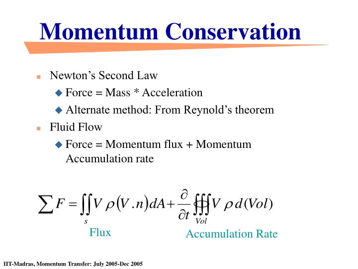
Momentum Conservation. Newton’s Second Law Force = Mass * Acceleration Alternate method: From Reynold’s theorem Fluid Flow Force = Momentum flux + Momentum Accumulation rate. Flux. Accumulation Rate. 0. Example. Straight Pipe. Steady State. A 2 V 2. A 1 V 1. Assumption: No friction.

E N D
Momentum Conservation • Newton’s Second Law • Force = Mass * Acceleration • Alternate method: From Reynold’s theorem • Fluid Flow • Force = Momentum flux + Momentum Accumulation rate Flux Accumulation Rate
0 Example • Straight Pipe • Steady State A2 V2 A1 V1 • Assumption: No friction
1 2 Example • Flow in a straight pipe. Realistic case
0 r1=1g/cm3 d1=8cm • Steady State V1=5m/s d2=5cm Example • Problem: 5.32 d2,V2 d1,V1 1 2 h=58 cm
y x Weight of Fluid Example • Example 1 (bent pipe), page 47 r1,V1 By Area=A1 Area=A2=A1 Q Bx r2,V2
out in in out Example • Steady State • d/dt =0 • From Eqn of Conservation of Mass
Example V1 By Area=A1 Area=A2=A1 Q Bx V2
Example • Pipe with U turn P1,V1 F P2,V2 Use Gage Pressure! In case of gas, use absolute pressure to calculate density
Example N • “L” bend P1 E F Assume the force by the pipe on the fluid is in the positive direction P2 What will the force be, if the flow is reversed (a) in a straight pipe? (b) in a L bend?
Conservation of Mass X Y Example Pbm. 5.13 & 5.19 V2 r1 P2 r2 Vw P1 V1 Stationary CV
X Y Example Pressure difference? Pbm. 5.19 V1=-3 m/s V2=0 m/s Vw=Velocity of Sound in water V2 r1 r2 Vw P2 P1 V1 Stationary CV ~ 41 atm
y x Example V2=? Pbm. 5.1,5,3 V1=6 m/s 0.6 m 1.2 m
Momentum Conservation • Angular Momentum • In a moving system • Torque = Angular Momentum flux + Angular Momentum Accumulation rate Flux Accumulation Rate
Q Example • Example 4 in book • Find the torque on the shaft • In a moving system • Torque = Angular Momentum flux + Angular Momentum Accumulation rate
Q Example • Approach-1. Find effective Force in X direction • Find the moment of Force • Assume: No frictional loss, ignore gravity, steady state, atmospheric pressure everywhere
Example • Approach-2. Using conservation of angular momentum • Stationary CV
Example • Consider a jet hitting a moving plate • After 1 second • Vnoz water has entered into the CV • Plate has moved by Vplate • In a control volume which moves with the plate, Vnoz-Vplate water has entered the CV (and exited at the bottom)
Consider plate moving @ half Vnoz, alpha = 180 degrees Example
Example • Pbm 5.24 • Thickness of slit =t, vol flow rate =Q, dia of pipe=d, density given • Ignore gravity effects 3ft 6ft Flux Accumulation Rate
Example 1 3ft • Pbm 5.31 • P1, P2, density, dia, vol flow rate given 2 • Calculate velocity at 1 (=2)
Friction Loss (Viscous) Mechanical Work done by the system Heat Work done by pressure force Energy Conservation
Energy Conservation • No Frictional losses • Incompressible • Steady • No heat, work • No internal energy change
Example • Flow from a tank Dia = d1 1 h1 0 2 Dia = d2 • Pressure = atm at the top and at the outlet h3 3 • Velocity at 1 ~ 0 • Toricelli’s Law • Sections 2 and 3
Example • How long does it take to empty the tank? • What if you had a pipe all the way upto level 3? Dia = d1 1 h1 0 2 Dia = d2 h3 3 • Pressure @ section 2 != atm • Pressure @ section 3 = atm
Example • What if you had a pipe all the way upto level 3? Dia = d1 1 h1 0 2 Dia = d2 h3 3 • More flow with the pipe • Turbulence, friction • Unsteady flow • Vortex formation
Example Height is known • Moving reference; Aircraft 60 km/h • Find P and r (eg from tables) 150 km/h • Flight as Reference 1 2 3
Flow through a siphon vs constriction h3 h1 h2 1 2
Example • Pbm. 6.4 • Steady flow through pipe , with friction • Friction loss head = 10 psi • Area, vol flow rate given • Find temp increase • Assume no heat transfer
Example D2 • Pbm. 6.10 • Fluid entering from bottom, • exiting at radial direction • Steady, no friction t P2=atm h2 D1 • Find Q, F on the top plate P1=10 psig
Example F y D1 P1=10 psig • If the velocity distribution just below the top plate is known, then P can be found using Bernoulli’s eqn
Modifications to Eqn • Unsteady state, for points 1 and 2 along a stream line
R 1 H L 2 D Draining of a tank • We can obtain the time it takes to drain a tank • (i) Assume no friction in the drain pipe • (ii) Assume you know the relationship between friction and velocity • Le us take that the bottom location is 2 and the top fluid surface is 1 • Incompressible fluid
Draining of a tank: Quasi steady state • Quasi steady state assumption • Velocity at fluid surface at 1 is very small • i.e. R >> D • No friction : L is negligible • P1 = P2 = Patm
Draining of a tank: Quasi steady state • Original level of liquid is at H = H0 • Integrating above equation from t=0, H=H0 to t=tfinal, H =0, we can find the efflux time
Draining of a tank: Unsteady state • BSL eg.7.7.1 • At any point of time, the kinetic + potential energy of the fluid in tank is converted into kinetic energy of the outgoing fluid • We still neglect friction • Potential Energy of a disk at height z and thickness dz
Draining of a tank: Unsteady state • Also, using continuity equation • Substituting, you get a 2nd order non linear ODE with two initial conditions. Please refer to BSL for solution
R 1 H L 2 D Draining of a tank (accounting for friction) • What if the flow in the tube is laminar and you want to account for friction? • Bernoulli’s eqn is not used (friction present) • Continuity • Hagen-Poiseuille’s eqn
Draining of a tank (accounting for friction) • Substituting and re arranging, • Integrating with limits • Note: The answer is given in terms of diameter of tube, so that it is easier to compare with the answer given in the book
Example • A1,A2, initial height h1 known • A1 >> A2 1 L • Consider section 3 and 2 h1 3 2 • Pseudo Steady state ==> Toricelli’s law
Example • Rearranging and solving, we get • As t increases, the solution approaches the Toricelli’s equation
Appendix:Example • Oscillating fluid in a U-tube 1 • Let h=h1-h2 h1 2 h2 L3
Appendix:Example • Blood Flow in vessels • Minimization of ‘work’ • Murray’s Law: • Laminar Flow, negligible friction loss (other than that due to viscous loss in laminar flow) , steady • Turbulent, pulsating flow • Assume
Appendix:Example • If the ratio of ‘smaller’ to larger capillary is constant • And Metabolic requirement =m= power/volume • Work for maintaining blood vessel • Total work • Optimum radius