Signal Detection and Processing Techniques

1. Signal Detection and Processing Techniques IITM-WPW-VKA

2. The essence of frequency analysis is the representation of a signal as superposition of sinusoidal components. • In practical applications, where only a finite length of data is available, we cannot obtain a complete description of the adopted signal model. • Therefore, an approximation (estimate) of the spectrum of the adopted signal model is computed. The quality of the estimate depends on • How well the assumed signal model represents the data. • What values we assign to the unavailable signal samples. • Which spectrum estimation method we use. • Clearly, a meaningful application of spectrum estimation to practical problems requires sufficient apriori information, understanding of the signal generation process, knowledge of theoretical concepts, and experience.

3. Signal Detectability and Pulse Compression • The efficiency of the radar system depends on how best it can identify the echoes in the presence of noise and unwanted clutter. • The important parameters from the system point of view influence the radar returns are the average power of transmission and the antenna aperture size. • Signal detectability is a measure of the radar performance in terms of transmission parameters.

4. Received signal power Psig to the uncertainty Pn in the estimate of the noise power after averaging Ae effective antenna areaPt peak power transmitted  pulse length,PRF pulse repetition frequency Pave = PtPRF average Tx powerBrec receiver band-width Ts effective system noise temp. Nc No. of samples coherently added Ninc number of resulting sums which are incoherently averaged c 1/Bsig correlation time of the scattering medium for the wavelength used t total integration time h range or height h height resolution.

5. Average power is the important parameter for the strong returns and this is function of pulse length. • Short pulses are required for good range resolution, and the shorter length of Inter pulse period (IPP) generates the problem of range ambiguity. (Therefore maximum limit on the PRF is restricted due to the above problems) • Pulse compression and frequency stepping are techniques which allow more of the transmitter average power capacity to be used without sacrificing range resolution. • A pulse of power P and duration  is in a certain sense converted into one of power nP and duration /n. • In the frequency domain compression involves manipulating the phases of the different frequency components of the pulse. • In the time domain a pulse can be compressed via phase coding, especially binary phase coding, a technique which is particularly amenable to digital processing techniques. • Since frequency is just the time derivative of phase, either can be manipulated to produce compression. • Phase coding has been used extensively in atmospheric radars and in commercial & military applications.

6. Phase coded waveform . +1 + + + + - - - Pulse compression Barker codes • These were first discussed by Barker (1953) and have been used in Ionospheric incoherent scatter measurements. The distinguishing feature of these codes is that, the range side-lobes have a uniform amplitude of unity. • The compression process only works, if the correlation time of the scattering medium is substantially longer than the full-uncompressed length of the transmitted pulse -1 Binary phase coded signal ACF 14 

7. 16 + + + - + + - + + + + - - - + - EDE2 ACF of pulse 1 8 -8 Complementary code pairs • Barker codes have range side lobes which are small, but which may still cause problems in MST applications. • Ideally a codes which supports high compression ratios (long codes) to get the possible altitude resolution. • Complementary phase codes are binary in their simplest form and they usually come in pairs. • They are coded exactly as Barker codes, by a matched filter whose impulse response is the time reverse of the pulse. • The range side lobes of the resulting ACF output for each pulse will generally be larger for a barker code of comparable length. • when the two pulses are complementary pair have the property that their side lobes are equal in magnitude but opposite in sign, so that when outputs are added the side lobes exactly cancel, leaving only the central peak. + + + - + + - + - - - + + + + - + ED1D ACF of pulse 1 16 8 32 -8 32 Sum of ACFs 16 0 32

8. Input Output IMS A100 Modified transversal filter architecture C(30) C(0) C(1) C(31) Z-1 Z-1 Decoding

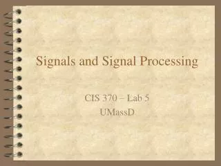
9. Signal Processor On-line/Off-line Processing I-Channel Windowing Decoder (I&Q) Coherent Integrator Normalization Q-Channel Time Series Fourier Analysis & Power Spectrum Incoherent Averaging Spectrum Cleaning Noise level Estimation Power Spectrum Moments UVW Zonal, Meridional, Vertical wind velocity Total Power, Mean Doppler, Doppler Width Off-line Processing Processing steps for extraction of parameters Signal and Data Processing

10. Coherent Integration • The detected quadrature signals are coherently integrated for many pulse returns which lead to an appreciable reduction in the volume of the data to be processed and an improvement in the SNR. • The coherent integration is made possible because of the over sampling of the Doppler signal resulting from the high PRF relative to the Doppler frequency. • In other words, the coherence time of the scattering process c is much greater than the sampling interval given by the inter pulse period tp. • The operation of coherent integration amounts to applying a low pass filter, whose time-domain representation is a rectangular window of Ti duration. • The signal spectrum is weighted by that of the integration filter sin2x/x2, where x = fTi and f is the Doppler shift in Hz. • The sampling operation at the integration time interval of Ti leads to frequency aliasing with signal power at frequencies f (m/Ti), where m is any integer, added to that at f.

11. In the case of a flat spectrum, the filtering and aliasing balance each other and white noise still looks white, with no tapering at window edges. • On the other hand, a signal peak with Doppler shift of 0.44/Ti Hz, near the edge of the aliasing window, will be attenuated by 3 dB by the filter function, whereas a peak near the center of the spectrum will be almost unaffected. • One should, therefore, be conservative in choosing Ni for coherent integration so as to ensure that all signals of interest are in the central portion of the post-integration spectrum. • The objective is to measure a signal x(n) of duration of N samples, n = 0,1, . . . . N-1. The measurement can be performed repeatedly. A total of M such measurements are performed and the results are averaged by the signal averaging. Let the results of the mth measurements, for m = 1,2, . . . M, are the samples. where x(n) and (n) corresponds to signal and noise respectively.

12. ym(t) ym(n) A/D Converter Memory After measurements • Integrates (average) the results of the M measurements • The result of the averaging operation may be expressed as • Assuming nm (n) to be mutually uncorrelated; that is, E[ nm(n) nl(n) ] = sn2 dml, • The variance of the averaged noise

13. therefore signal to noise ratio (SNR) is improved by a factor of M. • To increase the SNR, the number of coherent integration should be selected as large as possible within which the received signals are phase coherent with each other. • There are two cases that make the integration time finite • 1. movement of scatterers relative to each other within the radar sampling volume. • 2. the mean motion of scatterers relative to the radar due to background wind fields. • The relative motion of scatterers is estimated by a correlation time, which is defined as a half-power width of an auto correlation function of the received signal.

14. It depends on the radar wavelength, antenna beamwidth and altitude. • Inverse of the coherent integration time corresponds to half of the maximum frequency range of the Doppler spectra. • Therefore integration time should be so selected as to unambiguously determine the maximum radial wind velocity. • This limits the length of coherent integration. Normalization • The input data is to be normalized by applying a scaling factor corresponding to the operation done on it. • This will reduce the chance of data overflowing due to any other succeeding operation.

15. Normalization • The Normalization has following components. • a. sampling resolution of ADC • b. scaling due to pulse compression in decoder • c. scaling due to coherent integration • d. scaling due to number of FFT points. • if v - ADC bit resolution ( 10/16384), w - Pulse width in microsecond, M -Number of IPP integrated = Integrated time /inter pulse period, N - Number of FFT points, then the Normalization factor • The complex time series { Ii , Qi where i = 0, . . ,N-1} at the output of the signal processor is scaled as

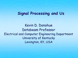
16. Amp Picket fence effect Leakage F() Amp f1 1 Cosine wave impulse 0.6 1 2 3 0 4 5 6 7 freq Independent Filters W() Power response Power +f -f FT of Rectangular Window 1 0.4 0 1 2 3 4 5 6 7 Frequency F() * W() f1 +f -f Windowing • It is well known that the application of FFT to a finite length data gives rise to leakage and picket fence effects.

17. Weighting the data with suitable windows can reduce these effects. • However the use of the data windows other than the rectangular window affects the bias, variance and frequency resolution of the spectral estimates. • In general variance of the estimate increases with the uses of a window. An estimate is said to be consistent if the bias and the variance both tend to zero as the number of observations is increased. • Thus, the problem associated with the spectral estimation of a finite length data by the FFT techniques is the problem of establishing efficient data windows or data smoothing schemes. • Characteristics of a window • It is desired that a window, f(t), has the following properties. • 1. f(t) is real and non-negative. • 2. f(t) is an even function, i.e., f(t) = f(-t). • 3. f(t) should attain its maximum at t=0, i.e., | f(t) | < f(0) for all t. • 4. Main lobe width should be as small as possible. • 5. The Maximum sidelobe level should be as small as possible relative to the main lobe peak. • 6. The mainlobe should contain a large part of the total energy. • 7. If the mth derivative of f(t) is impulsive, then the peak of the side-lobes of | F(w) | decays asymptotically as 6m dB/octave.

18. Rectangular ( Box Car ) window Window is defined by and its Fourier transform • Bartlet Window Window is defined by and its Fourier transform • Hanning Window Window is defined by and its Fourier transform

19. Hamming WindowWindow is defined by and its Fourier transform • COS3 Window window is defined by and its Fourier transform

20. BlackmanWindow Window is defined by and its Fourier transform is • Computation of window parameters The important window parameters which are useful in selecting an appropriate window for a particular application, which are 1. Variance compensation factor 2. Dispersion factor

21. 3. Total energy 4. Major lobe energy contents (MLE). 5. Half power bandwidth (HPBW) 6. W = major lobewidth/ major lobe width of rectangular window. 7. BW = Half power bandwidth/ Half power bandwidth of rectangular window. 8. coherent gain 9. Rate of fall of sidelobe levels (RFSL). 10. Peak sidelobe level (PSLL). 11. Degradation loss L, is the reciprocal of the dispersion in dB. Data window h Q E MLE SLL W BW G L RFSL (dB) (dB/Oct) ( % ) Rectangular 1.0 1.0 2.0 90.282 -13.26 1.0 1.0 1.0 0.0 -6 Hanning 1.50 0.375 0.75 99.9485 -31.48 2.0 1.63 0.5 -1.76 -6 Hamming 1.363 0.397 0.795 99.9632 -42.62 2.0 1.48 0.54 -1.34 -6 cosine3 1.735 0.313 0.625 99.9925 -39.30 2.50 1.81 0.42 -2.39 -24 Bartlet 1.333 0.333 0.6667 99.7057 -26.53 2.0 1.40 0.5 -1.25 -12 Blackman 1.727 0.305 0.609 99.9989 -58.12 3.0 1.86 0.42 -2.37 -18

22. A window that yields • small values of variance compensation factor, dispersion factor, total energy, peak sidelobe level, W and BW,and a large value of major lobe energy content is desirable in spectral estimation via FFT. • However a decrease in peak sidelobe level is associated with an increase in major lobewidth and, hence, a corresponding increase in the loss of frequency resolution. • The energy of window is an important parameter since the variance of the smoothed spectral estimate is proportional to E. • But the variance of the estimate is a measure of its reliability; smaller the value, higher is the reliability of the estimate. • Thus, the selection of data window for spectral estimation is a judicious compromise among the various parameters described above.

23. Weighting the data with suitable windows can reduce leakage. • Tapering is another name for the data windowing operation in the time domain. • Single taper smoothed spectrum estimates are plagued by a trade-off between the variance of the estimate and the bias caused by spectral leakage. • Applying a taper to reduce bias discards data, increasing the variance of the estimate. • Using a taper also unevenly samples the record. Single taper estimators, which are less affected by leakage, not only have increased variance but also can misrepresent the spectra of non-stationary data. • So as long as only a single data taper is used, there will be a trade-off between the resistance to spectral leakage and the variance of a spectral estimate.

24. Single taper spectral estimates have relatively large variance (increasing as a large fraction of data is discarded and the bias of the estimate is reduced) and are inconsistent estimates (i.e., the variance of the estimate does not drop as one increases the number of data). • To counteract this, it is conventional to smooth the single taper spectral estimate by applying a moving average to the estimate. • This reduces the variance of the estimate but results in a short - range loss of frequency resolution and therefore an increase in the bias of the estimate. • An estimate is to be consistent if the bias and the variance both tend to zero as the number of observations is increased. • Thus, the problem associated with the spectral estimation of a finite length data by the FFT techniques is the problem of establishing efficient data windows or data smoothing schemes.

25. Multitaper spectral analysis technique find wider applications in the signal analysis • First, the data are multiplied by not one, but several leakage - resistant tapers. This yields several tapered time series from one record. • Taking the DFTs of each of these time series, several “eigen spectra” are produced which are averaged to form a single spectral estimate. • There are a number of Multitapers that have been proposed. • Some of them are Slepian tapers, Discrete Prolate Spheroidal sequences, Sinusoidal Tapers, etc, • The central premise of this multitaper approach is that if the data tapers are properly designed orthogonal functions, then, under mild conditions, the spectral estimates would be independent of each other at every frequency.

26. 1 N Data Record 1 N Taper 1 1 N Periodogram A V E R A G E R 1 N Taper 2 1 N Periodogram 1 N Taper M 1 N Periodogram Final Estimate • Averaging would reduce the variance while proper design of full - length windows would reduce bias and loss of resolution. • The pictorial description of the multitaper approach to power spectrum estimation is as shown in Figure.

27. The multiple tapers are constructed so that each taper samples the time series in a different manner while optimizing resistance to spectral leakage. • The statistical information discarded by the first taper is partially recovered by the second taper, the information discarded by the first two tapers is partially retrieved by the third taper, and so on. • Only a few lower-order tapers are employed, as the higher - order tapers allow an unacceptable level of spectral leakage. • One can use these tapers to produce an estimate that is not hampered by the trade - off between leakage and variance that plagues single-taper estimates.

28. ; n = 1,2,…,N ; k=1,2,…,K Sinusoidal Multitaper • The continuous time minimum bias tapers are given as and its Fourier Transform as • The discrete analogs of the continuous time minimum bias tapers are called sinusoidal tapers. The nth sinusoidal taper is given by

29. k=1,2,..., K Where the amplitude term on the right is normalization factor that ensures orthonormality of the tapers. These sine tapers have much narrower main-lobe and much higher side-lobes. Thus they achieve a smaller bias due to smoothing by the main lobe, but at the expense of side-lobe suppression. Clearly this performance is acceptable if the spectrum is varying slowly. The kth sinusoidal taper has its spectral energy concentrated in the frequency bands.

30. Sinusoidal Multitaper

36. Fourier analysis • Spectral analysis is connected with characterizing the frequency content of a signal. • A large number of spectral analysis techniques are available in the literature. This can be broadly classified in to non-parametric or Fourier analysis based method and parametric or model based methods. • Fourier proposed that any finite duration signal, even a signal with discontinuities, can be expressed as an infinite summation of harmonically related sinusoidal component • FFT applied to complex time series {(Ii, Qi), i = 0,1, . . . ,N-1} to obtain complex frequency domain spectrum { (Xi, Yi), i = 0, . . . . , N-1} • Power Spectrum Power spectrum is calculated from the complex spectrum as

39. Incoherent Integration ( Spectral averaging) • Incoherent integration is the averaging the power spectrum number of times. where m is the number of spectra integrated. • The advantage of incoherent integration is that it improves the detectability of Doppler spectrum. The detectability is defined as where PS is peak spectral density of the signal spectrum, and sS+N is the standard deviation of spectral densities. • When fluctuations of the signal spectral density is much smaller than that for noise, then • The noise spectral density has a c2 distribution, because the noise spectral density is a summation of square of real and imaginary components of amplitude spectrum which are assumed to have Gaussian distribution.

40. The mean value m and standard deviation s of the c2 distribution becomes • For a single spectrum sN is equal to PN. • When Doppler spectra are averaged m times, the mean values of spectral densities of both the signal and noise are not changed. • But sN / PN becomes 1/Ö(m). • as m times integration of the noise produces a c2 distribution and as a result D is increased by Ö(m).

41. IITM-WPW-VKA

42. -fmax 0 fmax Power spectrum cleaning • Due to various reasons the radar echoes may get corrupted by ground clutter, system bias, interference, image formation etc.. • The data is to be cleaned from these problems before going for analysis. N/2 corresponds to zero frequency. • Spikes (glitches) in the time series will generate a constant amplitude band all over the frequency bandwidth. • Constant frequency bands will form in the power spectrum by the interference generated in the system or due to extraneous signal.

43. Noise level estimation • There are many methods adapted to find out the noise level estimation. • Basically all methods are statistical approximation to the near values. • The method implemented here is based on the variance decided by a threshold criterion, Hildebrand and Sekhon (1974). • This method makes use of the observed Doppler spectrum and of the physical properties of white noise; it does not involve knowledge of the noise level of the radar instrument system and is now widely used in atmospheric radar noise threshold estimation and removal.

46. The noise level threshold shall be estimated to the maximum level L, such that the set of Spectral points below the level S, nearly satisfies the criterion, Step 1: Reorder the spectrum { Pi, i = 0, . . . N-1} in ascending order to form. Let this sequence be written as{ Ai, i = 0, . . . N-1} and Ai < Aj for i < j Step 2: compute Where M is the number of spectra that were averaged for obtaining the data. Step 3:

47. Moments Estimation • The extraction of zeroth, first and second moments is the key reason for on doing all the signal processing and there by finding out the various atmospheric and turbulence parameters in the region of radar sounding. The basic steps involved in the estimation of moments, Woodman (1985) are given below. • Step 1. • Reorder the spectrum to its correct index of frequency (ie. -fmaximum to +fmaximum) in the following manner. • Spectral index 0 1 N/2 N-1 ambiguous freq. -fmaximum Zero freq. +fmaximum • Step 2: • Subtract noise level L from spectrum • Step 3: • i) Find the index l of the peak value in the spectrum, • ii) Find m, the lower Doppler point of index from the peak point. • iii) Find n the upper Doppler point of index from the peak point

48. P P  fd • Step 4:The moments are computed as • represents zeroth moment or Total Power in the Doppler spectrum. • represents the first moment or mean Doppler in Hz • represents the second moment or variance, a measure of dispersion from central frequency.

49. Sample Doppler spectra for a few range gates showing 5 candidate-peaks per range gate that form the basis for the adaptive technique of signal detection. IITM-WPW-VKA

50. (a) Height profiles of Doppler power spectra observed on 10 July 2002 using the 10o east radar beam when the SNR is low. (b) Mean Doppler Velocity-Height profile extracted from the spectra shown in (a) using the conventional peak detection method (dotted line) and the adaptive moments extraction technique (solid line). IITM-WPW-VKA