Download
1 / 32
320 likes | 482 Views
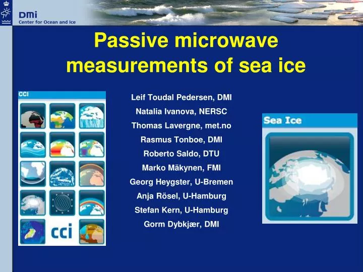
Passive microwave measurements of sea ice. Leif Toudal Pedersen, DMI Natalia Ivanova , NERSC Thomas Lavergne , met.no Rasmus Tonboe , DMI Roberto Saldo, DTU Marko Mäkynen , FMI Georg Heygster , U-Bremen Anja Rösel , U-Hamburg Stefan Kern, U-Hamburg Gorm Dybkjær, DMI.

E N D
Passive microwavemeasurements of seaice Leif Toudal Pedersen, DMI Natalia Ivanova, NERSC Thomas Lavergne, met.no Rasmus Tonboe, DMI Roberto Saldo, DTU Marko Mäkynen, FMI Georg Heygster, U-Bremen Anja Rösel, U-Hamburg Stefan Kern, U-Hamburg Gorm Dybkjær, DMI
Algorithmevaluation • Sensitivity to atmosphere • Open water dataset • Simulated data incl RTM corrected TBs from RRDP • Met/ocean data screening • Sensitivity to emissivity variations • 100% ice dataset • Simulated data • Snow/ice/atmosphere data screening • Summer performance (snow/ice melt and melt-ponds) • SMMR vs SSMI vs AMSR-E performance • Thin ice performance • Potential resolution
Convergence at ca. 100% • Deformation field between 20100109 and 20100110 from ENVISAT ASAR WSM Dataset of daily data from June 2007 to present exists from PolarView/MyOcean at DTU Red: Convergence Blue: Divergence
Algorithm portefolio • Some new algorithms (combinations) wereadded
Artificial data combinations • Some algorithms have cut-offs/non-linearities that does not allow a thorough validation at only 0 and 100% ice. • We have generated a dataset of 15% ice and 85% ice using our 0% and 100% • SIC15 = 0.85*SIC0(t)+0.15*SIC100(avgFY) • SIC85 = 0.85*SIC100(t)+0.15*SIC0(avgW)
NT2 • Has a bias of 10-15% at 85% ice, so a lot of datapoints at 85% aretruncated at 100% • Real performance at SIC=85% is somethinglike 10% (estimated from SSMI resultsthatarelessbiased)
Weather filters • Weather filters aresupposed to removeopenwater points that show icebecause of atmosphericinfluence (set SIC=0) . • We have establishedfurtherartificialdatasets at 20, 25 and 30% SIC for testing of weather filters.
Weather filters ICE ICE ICE ICE
Weather filters • Tested and we found that they remove ice up to sic>25% • We therefore generated a subset of RRDP with appended ERA Interim • Calculated corrections of TBs due to wind, water vapour and temp. Tried CLW but it was bad • Applied all algorithms to this new set
Atmosphericcorrection Upwelling + surface contrib. Reflected downwelling contrib. Reflected sky contrib. Tap = εTs + n
AtmosphericcorrectionStdev at SIC=0before and after Atm correctionStill no WF
Atmospheric correction using RTM • CF algorithm before and after RTM correction with ERA INTERIM
IOMASA IRT • Simple assimilation of TB (0Dvar) • RTM + surfaceemisivity forward model • Climatology as backgroundstate • Usingonly 6, 10, 18, 23 and 37 • Not 89 pt. • No SSMI pt
AMSR - February 4, 2006 Ice concentration MY-fraction Ice temperature ”Error” Water Vapour Cloud liquid water Wind Speed SST
RRDP results, SIC=0 • Small RMS error • 1.71% • Small bias • -0.05%
CF(rtm) vsIOMASA(irt) for SIC=0 Iceconc in % Iceconc in fractions of 1 Stdev=2.50 (before atm 4.3) Stdev=1.71
Thin ice Use SMOS-ice product to identify extensive areas of thin ice (2010)
Concentration of 100% 20 cm ice Concentration of 100% 10 cm ice
SIC vs (1-OW)OW is melt ponds + leadsCombination of meltedsnow/icethatcausesoverestimation and OW thatdoes the opposite
Data format for validation dataSimple comma separated ASCII text file (.csv)
Conclusions • Weselect a relatively simple and linear algorithm (CF or OSISAF) • Weperformatmosphericcorrection to TBs to reduce atm noise • Weapplydynamictie-points to accomodateresidual sensor drift and seasonalcycle in signatures
The end Thank you for your attention