Download

1 / 53
550 likes | 608 Views
Learn the basics of correlation and regression in statistical analysis to understand relationships between variables. Discover how to interpret data, hypothesis testing, and regression slope calculation.

E N D
Correlation and Regression The test you choose depends on level of measurement: Independent Dependent Test Dichotomous Continuous Independent Samples t-test Dichotomous Nominal Nominal Cross Tabs Dichotomous Dichotomous Nominal Continuous ANOVA Dichotomous Dichotomous Continuous Continuous Bivariate Regression/Correlation Dichotomous
Correlation and Regression • Correlation is a statistic that assesses the strength and direction of association of two continuous variables . . . It is created through a technique called “regression” • Bivariate regression is a technique that fits a straight line as close as possible between all the coordinates of two continuous variables plotted on a two-dimensional graph--to summarize the relationship between the variables
Correlation and Regression • For example: A sociologist may be interested in the relationship between education and self-esteem or Income and Number of Children in a family. Independent Variables Education Family Income Dependent Variables Self-Esteem Number of Children
Correlation and Regression • For example: • Research Hypothesis: As education increases, self-esteem increases (positive relationship). • Research Hypothesis: As family income increases, the number of children in families declines (negative relationship). Independent Variables Education Family Income Dependent Variables Self-Esteem Number of Children
Correlation and Regression • For example: • Null Hypothesis: There is no relationship between education and self-esteem. • Null Hypothesis: There is no relationship between family income and the number of children in families. Independent Variables Education Family Income Dependent Variables Self-Esteem Number of Children
Correlation and Regression • Let’s look at the relationship between income and number of children. • Regression will start with plotting the coordinates in your data (although you will hardly ever “plot” your data in reality). • The data: Case: 1 2 3 4 5 6 7 8 9 10 11 12 13 14 15 16 17 18 19 20 21 22 23 24 25 Children (Y): 2 5 1 9 6 3 1 0 3 7 7 2 4 2 1 0 1 2 4 3 0 1 2 5 7 Income 1=$10K (X): 3 4 9 5 4 12 14 10 1 4 3 11 4 9 13 10 7 5 2 5 15 11 8 3 2
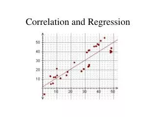
Correlation and Regression Y Plotted coordinates for income and children What do you think the relationship is? 1 2 3 4 5 6 7 8 9 10 X 1 2 3 4 5 6 7 8 9 10 11 12 13 14 15 Case: 1 2 3 4 5 6 7 8 9 10 11 12 13 14 15 16 17 18 19 20 21 22 23 24 25 Children (Y): 2 5 1 9 6 3 1 0 3 7 7 2 4 2 1 0 1 2 4 3 0 1 2 5 7 Income 1=$10K (X): 3 4 9 5 4 12 14 10 1 4 3 11 4 9 13 10 7 5 2 5 15 11 8 3 2
Correlation and Regression Y Plotted coordinates for income and children Is it positive? 1 2 3 4 5 6 7 8 9 10 X 1 2 3 4 5 6 7 8 9 10 11 12 13 14 15 Case: 1 2 3 4 5 6 7 8 9 10 11 12 13 14 15 16 17 18 19 20 21 22 23 24 25 Children (Y): 2 5 1 9 6 3 1 0 3 7 7 2 4 2 1 0 1 2 4 3 0 1 2 5 7 Income 1=$10K (X): 3 4 9 5 4 12 14 10 1 4 3 11 4 9 13 10 7 5 2 5 15 11 8 3 2
Correlation and Regression Y Plotted coordinates for income and children Is it negative? 1 2 3 4 5 6 7 8 9 10 X 1 2 3 4 5 6 7 8 9 10 11 12 13 14 15 Case: 1 2 3 4 5 6 7 8 9 10 11 12 13 14 15 16 17 18 19 20 21 22 23 24 25 Children (Y): 2 5 1 9 6 3 1 0 3 7 7 2 4 2 1 0 1 2 4 3 0 1 2 5 7 Income 1=$10K (X): 3 4 9 5 4 12 14 10 1 4 3 11 4 9 13 10 7 5 2 5 15 11 8 3 2
Correlation and Regression Y Plotted coordinates for income and children Is there no relationship? 1 2 3 4 5 6 7 8 9 10 X 1 2 3 4 5 6 7 8 9 10 11 12 13 14 15 Case: 1 2 3 4 5 6 7 8 9 10 11 12 13 14 15 16 17 18 19 20 21 22 23 24 25 Children (Y): 2 5 1 9 6 3 1 0 3 7 7 2 4 2 1 0 1 2 4 3 0 1 2 5 7 Income 1=$10K (X): 3 4 9 5 4 12 14 10 1 4 3 11 4 9 13 10 7 5 2 5 15 11 8 3 2
Correlation and Regression Y Plotted coordinates for income and children Well, the slope of the fitted line will tell us the nature of the relationship! 1 2 3 4 5 6 7 8 9 10 X 1 2 3 4 5 6 7 8 9 10 11 12 13 14 15 Case: 1 2 3 4 5 6 7 8 9 10 11 12 13 14 15 16 17 18 19 20 21 22 23 24 25 Children (Y): 2 5 1 9 6 3 1 0 3 7 7 2 4 2 1 0 1 2 4 3 0 1 2 5 7 Income 1=$10K (X): 3 4 9 5 4 12 14 10 1 4 3 11 4 9 13 10 7 5 2 5 15 11 8 3 2
Correlation and Regression Y What is the slope of a “fitted line?” The slope is the change in Y along the line as you go up one on X while following the line (rise over run). 1 2 3 4 5 6 7 8 9 10 Slope = 0, No relationship! 1 2 3 4 5 6 7 8 9 10 11 12 13 14 15
Correlation and Regression Y What is the slope of a “fitted line?” 1 2 3 4 5 6 7 8 9 10 0.5 1 Slope = 0.5, Positive Relationship! 1 2 3 4 5 6 7 8 9 10 11 12 13 14 15 The slope is the change in Y along the line as you go up one on X while following the line (rise over run).
Correlation and Regression Y What is the slope of a “fitted line?” Slope = -0.5, Negative Relationship! 1 2 3 4 5 6 7 8 9 10 0.5 1 1 2 3 4 5 6 7 8 9 10 11 12 13 14 15 The slope is the change in Y along the line as you go up one on X while following the line (rise over run).
Correlation and Regression • The mathematical equation for a line: Y = mx + b Where: Y = the line’s position on the vertical axis at any point X = the line’s position on the horizontal axis at any point m = the slope of the line b = the intercept with the Y axis, where X equals zero
Correlation and Regression • The statistics equation for a line: Y = a + bx Where: Y = the line’s position on the vertical axis at any point (value of dependent variable) X = the line’s position on the horizontal axis at any point (value of the independent variable) b = the slope of the line (called the coefficient) a = the intercept with the Y axis, where X equals zero ^ ^
Correlation and Regression • The next question: How do we draw the line??? • Our goal for the line: Fit the line as close as possible to all the data points for all values of X.
Correlation and Regression Y Plotted coordinates for income and children How do we minimize the distance between a line and all the data points? 1 2 3 4 5 6 7 8 9 10 X 1 2 3 4 5 6 7 8 9 10 11 12 13 14 15 Case: 1 2 3 4 5 6 7 8 9 10 11 12 13 14 15 16 17 18 19 20 21 22 23 24 25 Children (Y): 2 5 1 9 6 3 1 0 3 7 7 2 4 2 1 0 1 2 4 3 0 1 2 5 7 Income 1=$10K (X): 3 4 9 5 4 12 14 10 1 4 3 11 4 9 13 10 7 5 2 5 15 11 8 3 2
Correlation and Regression • How do we minimize the distance between a line and all the data points? • You already know of a statistic that minimizes the distance between itself and all data values for a variable--the mean! • The mean minimizes the sum of squared deviations--it is where deviations sum to zero and where the squared deviations are at their lowest value. (Y - Y-bar)2
Correlation and Regression • The mean minimizes the sum of squared deviations--it is where deviations sum to zero and where the squared deviations are at their lowest value. • Let’s take this principle and “fit the line” to the place where squared deviations (on Y) from the line are at their lowest value (across all X’s). • (Y - Y)2 • Y = line ^ ^
Correlation and Regression • There are several lines that you could draw where the deviations would sum to zero... • Minimizing the sum of squared errors gives you the unique, best fitting line for all the data points. It is the line that is closest to all points. • Y or Y-hat = Y value for line at any X • Y = case value on variable Y • Y - Y = residual • (Y – Y) = 0; therefore, we use (Y - Y)2 …and minimize that! ^ ^ ^ ^
Correlation and Regression • Let’s take this principle and “fit the line” to the place where squared deviations (on Y) from the line are at their lowest value (at any given X). Y = 9 ^ (Y - Y)2= (9 - 7)2 = 4 1 2 3 4 5 6 7 8 9 10 ^ Y = 7 ^ Y = 4 ^ (Y - Y)2= (2 - 4)2 = 4 Y = 2 1 2 3 4 5 6 7 8 9 10 11 12 13 14 15
Correlation and Regression Y Plotted coordinates for income and children The fitted line for our example has the equation: Y = 6 - .4X If you were to draw any other line, it would not minimize (Y - Y)2 ^ 1 2 3 4 5 6 7 8 9 10 ^ X 1 2 3 4 5 6 7 8 9 10 11 12 13 14 15 Case: 1 2 3 4 5 6 7 8 9 10 11 12 13 14 15 16 17 18 19 20 21 22 23 24 25 Children (Y): 2 5 1 9 6 3 1 0 3 7 7 2 4 2 1 0 1 2 4 3 0 1 2 5 7 Income 1=$10K (X): 3 4 9 5 4 12 14 10 1 4 3 11 4 9 13 10 7 5 2 5 15 11 8 3 2
Correlation and Regression ^ • We use (Y - Y)2 …and minimize that! • There is a simple, elegant formula for “discovering” the line that minimizes the sum of squared errors ((X - X)(Y - Y)) b = (X - X)2 a = Y - bX Y = a + bX • This is the method of least squares, it gives our least squares estimate and indicates why we call this technique “ordinary least squares” or OLS regression ^
Correlation and Regression In fact, this is the output that SPSS would give you for the data values: ^ Y = a + bX
Correlation and Regression Y ^ Considering that our line minimizes (Y - Y)2, where would the regression cross for two groups in a dichotomous independent variable? 1 2 3 4 5 6 7 8 9 10 X 0 1 0=Men: Mean = 6 1=Women: Mean = 4
Correlation and Regression Y The difference of means will be the slope. This is the same number that is tested for significance in an independent samples t-test. 1 2 3 4 5 6 7 8 9 10 ^ Slope = -2 ; Y = 6 – 2X X 0 1 0=Men: Mean = 6 1=Women: Mean = 4
Correlation and Regression • We’ve talked about the summary of the relationship, but not about strength of association. • How strong is the association between our variables? • For this we need correlation.
Correlation and Regression Y Plotted coordinates for income and children So our equation is: Y = 6 - .4X The slope tells us direction of association… How strong is that? ^ 1 2 3 4 5 6 7 8 9 10 X 1 2 3 4 5 6 7 8 9 10 11 12 13 14 15 Case: 1 2 3 4 5 6 7 8 9 10 11 12 13 14 15 16 17 18 19 20 21 22 23 24 25 Children (Y): 2 5 1 9 6 3 1 0 3 7 7 2 4 2 1 0 1 2 4 3 0 1 2 5 7 Income 1=$10K (X): 3 4 9 5 4 12 14 10 1 4 3 11 4 9 13 10 7 5 2 5 15 11 8 3 2
Correlation and Regression • To find the strength of the relationship between two variables, we need correlation. • The correlation is the standardized slope… it refers to the standard deviation change in Y when you go up a standard deviation in X.
Correlation and Regression 1 2 3 4 5 6 7 8 9 10 Example of Low Negative Correlation
Correlation and Regression 1 2 3 4 5 6 7 8 9 10 Example of High Negative Correlation
Correlation and Regression • The correlation is the standardized slope… it refers to the standard deviation change in Y when you go up a standard deviation in X. (X - X)2 • Recall that s.d. of x, Sx = n - 1 (Y - Y)2 • and the s.d. of y, Sy = n - 1 Sx • Pearson correlation, r = Sy b
Correlation and Regression • The Pearson Correlation, r: • tells the direction and strength of the relationship between continuous variables • ranges from -1 to +1 • is + when the relationship is positive and - when the relationship is negative • the higher the absolute value of r, the stronger the association • a standard deviation change in x corresponds with r standard deviation change in Y
Correlation and Regression • The Pearson Correlation, r: • The pearson correlation is a statistic that is an inferential statistic too. r - (null = 0) • tn-2 = (1-r2) (n-2) • When it is significant, there is a relationship in the population that is not non-existent!
Correlation and Regression ^ • Y = a + bX This equation gives the conditional mean of Y at any given value of X. • So… In reality, our line gives us the expected mean of Y given each value of X • The line’s equation tells you how the mean on your dependent variable changes as your independent variable goes up. Y ^ Y X
Correlation and Regression • As you know, every mean has a distribution around it--so there is a standard deviation. This is true for conditional means as well. So, you also have a conditional standard deviation. • “Conditional Standard Deviation” or “Root Mean Square Error” equals “approximate average deviation from the line.” SSE ( Y - Y)2 • = n - 2 = n - 2 Y ^ Y X ^ ^
Correlation and Regression • The Assumption of Homoskedasticity: • The variation around the line is the same no matter the X. • The conditional standard deviation is for any given value of X. • If there is a relationship between X and Y, the conditional standard deviation is going to be less than the standard deviation of Y--if this is so, you have improved prediction of the mean value of Y by looking at each level of X. • If there were no relationship, the conditional standard deviation would be the same as the original, and the regression line would be flat at the mean of Y. Y Original standard deviation Conditional standard deviation Y X
Correlation and Regression • So guess what? • We have a way to determine how much our understanding of Y is improved when taking X into account—it is based on the fact that conditional standard deviations should be smaller than Y’s original standard deviation.
Correlation and Regression • Proportional Reduction in Error • Let’s call the variation around the mean in Y “Error 1.” • Let’s call the variation around the line when X is considered “Error 2.” • But rather than going all the way to standard deviation to determine error, let’s just stop at the basic measure, Sum of Squared Deviations. • Error 1 (E1) = (Y – Y)2 also called “Sum of Squares” • Error 2 (E2) = (Y – Y)2 also called “Sum of Squared Errors” Y Error 1 Error 2 Y X
Correlation and Regression • Proportional Reduction in Error • To determine how much taking X into consideration reduces the variation in Y (at each level of X) we can use a simple formula: E1 – E2Which tells us the proportion or E1 percentage of original error that is Explained by X. • Error 1 (E1) = (Y – Y)2 • Error 2 (E2) = (Y – Y)2 Error 2 Y Error 1 Y X
Correlation and Regression r2 = E1 - E2 E1 = TSS - SSE TSS = (Y – Y)2 - (Y – Y)2 (Y – Y)2 r2 is called the “coefficient of determination”… It is also the square of the Pearson correlation Error 1 Y Error 2 Y X
Correlation and Regression • R2 • Is the improvement obtained by using X (and drawing a line through the conditional means) in getting as near as possible to everybody’s value for Y over just using the mean for Y alone. • Falls between 0 and 1 • Of 1 means an exact fit (and there is no variation of scores around the regression line) • Of 0 means no relationship (and as much scatter as in the original Y variable and a flat regression line through the mean of Y) • Would be the same for X regressed on Y as for Y regressed on X • Can be interpreted as the percentage of variability in Y that is explained by X. • Some people get hung up on maximizing R2, but this is too bad because any effect is still a finding—a small R2 only indicates that you haven’t told the whole (or much of the) story with your variable.
Correlation and Regression Back to the SPSS output: r2 (Y – Y)2 - (Y – Y)2 (Y – Y)2 71.194 ÷ 154.64 = .460
Correlation and Regression Q: So why did I see an ANOVA Table? A: Levels of X can be thought of like groups in ANOVA …and the squared distance from the line to the mean (Regression SS) is equivalent to BSS—group mean to big mean (but df = 1) …and the squared distance from the line to the data values on Y (Residual SS) is equivalent to WSS—data value to the group’s mean … and the ratio of these forms an F distribution in repeated sampling If F is significant, X is explaining some of the variation in Y. Y BSS WSS TSS Mean X
Correlation and Regression Using a dichotomous independent variable, the ANOVA table in bivariate regression will have the same numbers and ANOVA results as a one-way ANOVA table would (and compare this with an independent samples t-test). Y 1 2 3 4 5 6 7 8 9 10 BSS WSS TSS Mean = 5 ^ Slope = -2 ; Y = 6 – 2X 0 1 X 0=Men: Mean = 6 1=Women: Mean = 4
Descriptive: The equation for your line is a descriptive statistic. It tells you the real, best-fitted line that minimizes squared errors. Inferential: But what about the population? What can we say about the relationship between your variables in the population??? The inferential statistics are estimates based on the best-fitted line. Correlation and Regression Recall that statistics are divided between descriptive and inferential statistics.
Correlation and Regression • The significance of F, you already understand. • The ratio of Regression (line to the mean of Y) to Residual (line to data point) Sums of Squares forms an F ratio in repeated sampling. • Null: r2 = 0 in the population. If F exceeds critical F, then your variables have a relationship in the population (X explains some of the variation in Y). F = Regression SS / Residual SS Most extreme 5% of F’s
Correlation and Regression • What about the Slope (called “Coefficient”)? • The slope has a sampling distribution that is normally distributed. • So we can do a significance test. z -3 -2 -1 0 1 2 3