Download
1 / 57
580 likes | 690 Views
ISDN Networks and Applications Week 9. Dimensioning ATM Networks. Dr. Milosh V. Ivanovich e-mail: ivanovic@sub.net.au. $. The Question. The FUNDAMENTAL DILEMMA of Carriers and Service Providers : ??? How ??? to provide telecommunications services at minimal cost Subject to -

E N D
ISDN Networks and Applications Week 9 Dimensioning ATM Networks Dr. Milosh V. Ivanovich e-mail: ivanovic@sub.net.au
$ The Question • The FUNDAMENTAL DILEMMA of Carriers and Service Providers : ??? How ??? to provide telecommunications services at minimal cost Subject to - meeting Quality Of Service (QoS) requirements.
The Answer lies in ... • By applying sound NETWORK DESIGN principles fairness ... but Network Design has conflicting objectives !! economic QoS robustness
... Cleverly Exploiting ATM Network Features * Layered Network Architecture * Cell Priority Mgmt. Virtual Channel * VP Switching * VC Switching Virtual Path ATM network = a collection of partially separated logical networks. Physical
48 Bytes ... First a Brief ATM Refresher What is ATM ? • Asynchronous Transfer Mode • Cell switching (relay) • Fixed cell size of 53 octets • Connection-oriented technology
Why is it called “ASYNCHRONOUS” ? Idle Idle Idle • Cells are transmitted continuously (idle cells are inserted) • Supports bursty services, easily and efficiently • Header identifies information stream Idle Idle Cell Travel (full link rate) Headers
• Call Level • General – Connection Admission Control • point to point • broadcast – Call Set-up – Call Management (VC, VP) – Routing The Roles of ATM Traffic Management – QoS Class – Transfer Capability • Cell / Stream Level – Usage Parameter Control (Policing) – Congestion Control; Selective Discard – Traffic Shaping
ITU-T ATM Transfer Capability ATM Forum Service Category DBR - Deterministic Bit Rate CBR - Constant Bit Rate SBR - Statistical Bit Rate VBR-RT - Real Time Variable Bit Rate VBR-NRT - Non Real Time Variable Bit Rate ABT - ATM Block Transfer N/A ABR - Available Bit Rate ABR - Available Bit Rate N/A UBR - Unspecified Bit Rate ATM Transfer Capabilities ITU -T vs. ATM Forum
ATM Traffic Categories and Associated Applications Most Stringent QoS Requirement • Interactive Audio and Video (e.g. voice call, videoconference), Circuit Emulation: • CBR, QoS Class 1 • VBR-rt, QoS Class 1 • Transfer for immediate use (e.g. image transfer, n.r.t. guaranteed constant bit rate applications, maybe some TCP applications - TELNET, HTTP). • CBR, QoS Class 2/3 • VBR-nrt / ABR, QoS Class 2/3 • Transfer for later use (e.g most TCP applications - FTP, SMTP). • ABR / UBR, QoS Class 2 Least Stringent QoS Requirement
The Relationship Between Network Design and Dimensioning Network Design Structuring Dimensioning “the engineer” “the architect”
ATM Network Structuring • Key factors to consider : • Distribution of user population. • Traffic: expected volume, type, and time + geographical distributions. • Flexibility and scalability • Reliability • Low overall {switching, transmission} cost. • Guiding principles : • Choose a flat or layered switching architecture based on the above factors. • Pre-emptive traffic segmentation - maintain QoS.
ws ws ws ws ws S ws ws ws ws ws ws ws S S ws S S S ws ws ws ATM Network Structuring : Traffic Segregation VBR only CBR VBR Architecture A: Segregation Architecture B: Symmetry
ws ws ws VBR S CBR mesh ws ws ATM Network Structuring : an “ATM LAN” example • Mixing traffic types, while guaranteeing QoS may be achieved by: • Architectural Traffic Segregation • Traffic Shaping (Buffering!) and Policing VBR conns. • “Throwing raw bandwidth at the problem”
Traffic Management Buffering Bandwidth ATM Network Dimensioning Tradeoffs (for a given QoS)
What is the smallest bandwidth What is the predicted Cell (service rate) we can use to serve Loss Ratio (CLR) of a an SSQ fed by real traffic such that single server queue fed required CLR is met ? (for a given buffer size). by the modeled process? The Subject In a Nutshell : ... at the Burst Scale • ATM Network Dimensioning most commonly boils down to: Link Dimensioning CLR Prediction OR
Hierarchy of Time Scales Calls - Effective BW concept. - Multi-rate C.S. network. Bursts - Fluid flow models. - REM and RS. Cells - Randomness from phase independence.
The Call Scale : Effective Bandwidth • EB - Necessary to enable associating a “fixed” amount of bandwidth with each inherently variable bit-rate call. Can then model ATM network as a circuit switched network. • No single formula - EB depends on model used. • Example [GAN91], [KWC93] : We wish to determine the minimal required service rate CB(e) such that the probability PB=Pr{X > B} that the buffer occupancy (X) exceeds some level B is below e. The buffer is part of a Single Server Queue (SSQ) system fed by a Markov Modulated Rate Process (MMRP). Its complementary content distribution is approximately given by the exponential, • Q(x) = Pr{X > x} ~ he-zx Making the assumptions from [GAN91] (i.e. that h ~ 1) we get the Effective Bandwidth to be: • CB (e) = z -1(-log e / B)
Total of Service Times Number of Calls Average Service Time = Traffic Volume___ Period of Observation Average Traffic = The Call Scale : Review of some “Classical” Dimensioning Methods • The unit of traffic is the “erlang”, symbolised by “E” Some Definitions: Traffic Volume = Total of Service Times Traffic Volume = Number of Calls x Average Service Time Erlangs
Number of Calls__ Period of Observation x Average Service Time Average Traffic = Fundamental Relationship of Teletraffic Engineering (Avg. Departure Rate)-1 m-1 A Average Arrival Rate, l ... and what about “congestion” ?? A call encounters congestion or blocking if it can not proceed immediately due to lack of resources. * Call Congestion * Time Congestion * Traffic Congestion
The Call Scale : A Model of Repeat Call Attempts Often a blocked call’s initiator will try again ... All possible causes of Ineffective Attempts First Attempts Total Attempts S 1 - B B Successful Calls Repeat Attempts Ineffective Attempts R 1 - R Abandoned Calls
The Call Scale : Modelling a Loss System (Erlang-B) • The first step is to construct a State Transition Diagram. l l l l 2 n 0 1 m 3m 2m nm Use the “Cut” Method to obtain Balance Eqns. lP(0) = mP(1) lP(1) = 2mP(2)... up to n Define A = l / m ... (Offered Traffic, or alternatively, Utilisation).
Can we Really Use the Erlang-B Formula for ATM Network Dimensioning ? • YES, but ... • Only in one very special, and not very useful case: when all connections sharing the ATM bearer are of the same rate (“?!But the whole point of ATM is ...”) • For example, we could have 10 combined CBR and VBR VC connections, with EB = 2Mbit/s, sharing a 34Mbit/s ATM VP. • Blocking Probability would be = E (10, 34 / 2) • where E(*, *) is the Erlang-B Loss Function. • Conclusion : • WE NEED MORE SOPHISTICATED MODELS !
The Answer: Multi-rate Models • Basic Link Model for the Complete Sharing Policy • N different traffic classes accessing an ATM Tx link with cap. c Mbps • Arrival process for class i calls is Poisson, rate l i. • Holding time follows a general distribution function, mean 1/mi. • During the lifetime of a class i call, a constant rate denoted by ci, is allocated to it, and released immediately after its departure.
Basic Bandwidth Unit, BBU : • gcd is the “greatest common divisor”. • In broadband networks, typical BBUs may be 64kbps or 2.048Mbps. • Max. No. of available BBUs : • No. of BBUs required for class i : • System states defined by one quantity - the no. of occupied BBUs : m Kaufman and Roberts Recursive Solution • Exact algorithm - not an approximation. • Based on a mapping of the multi-dimensional state space into a one dimensional state space. • Uses “proper bandwidth discretisation”. • Prevents “State Explosion” by compressing many different states into one.
An Example : A Four Class System • Call Blocking Probabilities - note the UNFAIRNESS
An Example : A Four Class System (cont.) • Link utilisation sharing - related to UNFAIRNESS, note the under-utilisation for greater BW classes.
Equalisation and Fairness Issues • Basic link model for Trunk Reservation (TR). • Many different Connection Admission Control (CAC) strategies for achieving some form of fairness exist : complete sharing, partial sharing, class limitation, trunk reservation (TR). • For a comparson of such strategies, see [KW88]. • Briefly consider TR - one of the simplest and most effective methods to adjust/equalise call blocking. • Aim is to influence performance parameters such as call blocking pr.
Enhancements : Combined Call and Burst Scale Model • Similar to complete sharing model outlined on p25. • Tx link capacity c, N traffic classes (CBR & VBR). • CBR calls modelled at call level only. • VBR calls modelled at both burst and call levels. • Connection admission control and blocking behaviour is different for CBR and VBR calls: • CBR calls of class i • Must be accepted at CALL level. • And at BURST level. • VBR calls of class j • Must be accepted at CALL level only. Call Blocking Burst Blocking
The Burst (Stream) Scale - What is it? • A time scale typical of an: • ON/OFF source’s activity period, • Video Frame duration, • IP packet (carrying say a UDP datagram), • Or any other “interval” aggregating some cells, but not being as long as a call duration. • The discrete nature of cell arrivals can be ignored. • Instead, we focus on the incoming “stream” of cells. • Denoted by the continuous random variable An or A(t) representing the “amount of work” entering the system, • An used for discrete time modelling, • A(t) used for continuous time modelling .
The Burst Scale (cont.) • Time can either be modelled as : • Continuous: generally used for fluid flow based models. • Discrete: time divided into fixed-length sampling intervals. • Burst scale congestion - modelled by : • Burst scale loss, in the form of Rate Envelope Multiplexing (REM), and /or • Burst scale delay, in the guise of Rate Sharing (RS).
Three approaches for Link Dimensioning (and CAC) at the Burst Scale • Peak Allocation • Rate Envelope Multiplexing (REM) • Rate Sharing (RS)
Three approaches for Link Dimensioning (and CAC) at the Burst Scale (cont .)
Burst Scale Link Dimensioning Example • Want to dimension an ATM bearer, • Given 70 variable bit-rate 2 Mb/s connections, • How much capacity is needed? A Simple Solution: Peak Rate Allocation 70 x 2 = 140 Mb/s
Example Continued: Let’s Try REM • More information required for each connection: Peak (p) = 2 Mb/s, Mean (m) = 0.2 Mb/s • Assume On/Off Model for each connection so: Variance = (p - m) m = 1.8 x 0.2 = 0.36 • For 70 connections (linear superposition): Aggregate Mean = 70 x 0.2 = 14 Aggregate Variance = 70 x 0.36 = 25.2 • By the Central Limit Theorem, the Aggregate Traffic Rate (Mb/s) can be modelled by a Gaussian R.V. X : m = 14 and s2 = 25.2
REM Example - Continued • Minimize Required Link Bandwidth, B (Mb/s) • Subject to Bit Loss Ratio (BLR) < 10-5 • Where BLR is given by: BLR =E [( X - B )+ ] / E [X] Solution: (1) (X-B)+ = X-B if X >B and = 0 if X < B. (2) If X has density f(x) then:
REM Example - Continued Solution (cont.): (3) The Bit Loss Ratio is thus given by (4) Using the bisection algorithm, this equation is then numerically solved (e.g. use C++ program, or tool such as Mathematica): Bmin = 32.485376Mb/s.
Rate Sharing • More complex to model because : • Large buffers as well as bandwidth is considered, • Now correlation is important. • Traffic Modelling • Queueing Theory & Simulation • Real traffic traces • Two approaches: Classical and Direct.
Gamma Loss Prediction Tool : SSQ Dimensioning by the Classical Method Aim: Find Minimum service rate Subject to CLR Input: * Queue information (service, buffer) * Traffic model or trace Method: Bisection service rate Compute Cell Loss Rate (CLR) Find new service rate CLR
Autocorrelation of a Traffic Stream • Low autocorrelation • Low dependence between traffic arriving in intervals separated in time. • High autocorrelation • High dependence between traffic arriving in intervals separated in time.
100 80 Utilisation % 60 40 20 0 100 1,000 10,000 100,000 Buffer Size (cells) Real Life Example of RS versus REM (1) Link Utilisation vs. Buffer Size Measured Ethernet TRAFFIC - Loss Probability = 1/10,000 Rate Sharing REM
RS REM Real Life Example of RS versus REM (2) Link Utilisation vs. Buffer Size VBR Video TRAFFIC (MPEG) Loss Probability=1/10,000 70 60 50 40 Utilisa tion % 30 20 10 0 100 1,000 10,000 100,000 Buffer Size (cells)
Critical Statistical Characteristics of a Traffic Process • Mean, • Variance, • Autocovariance Sum or Autocovariance Integral (equal to the Asymptotic Variance Rate).
The Variance v=Autocovariance Integral -5.0 -4.0 -3.0 -2.0 -1.0 0.0 1.0 2.0 3.0 4.0 5.0 Arrival Process Autocovariance Sum / Integral Lag
Common SRD Traffic Models ... • Bernoulli Process • Geometric (or Binomial) Batch Process • On-Off • n-state Markov Modulated Processes • Gaussian
But what if the Autocovariance sum is infinite? LONG RANGE DEPENDENCE (LRD) otherwise known as SELF-SIMILAR (FRACTAL) TRAFFIC autocorrelation LRD SRD lag