Download

1 / 51
550 likes | 854 Views
Chapter 7. Statistical Intervals Based on a Single Sample. Weiqi Luo ( 骆伟祺 ) School of Software Sun Yat-Sen University Email : weiqi.luo@yahoo.com Office : # A313. Chapter 7: Statistical Intervals Based on A Single Sample. 7.1. Basic Properties of Confidence Intervals

E N D
Chapter 7. Statistical Intervals Based on a Single Sample Weiqi Luo (骆伟祺) School of Software Sun Yat-Sen University Email:weiqi.luo@yahoo.com Office:# A313
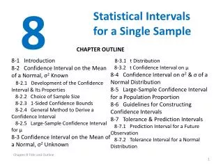
Chapter 7: Statistical Intervals Based on A Single Sample • 7.1. Basic Properties of Confidence Intervals • 7.2. Larger-Sample Confidence Intervals for a Population Mean and Proportion • 7.3 Intervals Based on a Normal Population Distribution • 7.4 Confidence Intervals for the Variance and Standard Deviation of a Normal Population
Chapter 7 Introduction • Introduction • A point estimation provides no information about the precision and reliability of estimation. • For example, using the statistic X to calculate a point estimate for the true average breaking strength (g) of paper towels of a certain brand, and suppose that X = 9322.7. Because of sample variability, it is virtually never the case that X = μ. The point estimate says nothing about how close it might be to μ. • An alternative to reporting a single sensible value for the parameter being estimated is to calculate and report an entire interval of plausible values—an interval estimate or confidence interval (CI)
7.1 Basic Properties of Confidence Intervals • Considering a Simple Case Suppose that the parameter of interest is a population mean μ and that • The population distribution is normal. • The value of the population standard deviation σis known • Normality of the population distribution is often a reasonable assumption. • If the value of μis unknown, it is implausible that the value of σwould be available. In later sections, we will develop methods based on less restrictive assumptions.
7.1 Basic Properties of Confidence Intervals • Example 7.1 Industrial engineers who specialize in ergonomics are concerned with designing workspace and devices operated by workers so as to achieve high productivity and comfort. A sample of n=31 trained typists was selected , and the preferred keyboard height was determined for each typist. The resulting sample average preferred height was80.0 cm. Assuming that preferred height is normally distributed with σ=2.0 cm. Please obtain a CI for μ, the true average preferred height for the population of all experienced typists. Consider a random sample X1, X2, … Xn from the normal distribution with mean value μ and standard deviation σ . Then according to the proposition in pp. 245, the sample mean is normally distribution with expected value μ and standard deviation
7.1 Basic Properties of Confidence Intervals • Example 7.1 (Cont’) we have
7.1 Basic Properties of Confidence Intervals • Example 7.1 (Cont’) True value of μ (Fixed) CI (Random) The CI of 95% is: Interval number with different sample means (1) (2) (3) (4) (5) (6) (7) Interpreting a CI: It can be paraphrased as “the probability is 0.95 that the random interval includes or covers the true value of μ. (8) (9) … (10) (11)
7.1 Basic Properties of Confidence Intervals • Example 7.2 (Ex. 7.1 Cont’) The quantities needed for computation of the 95% CI for average preferred height are δ=2, n=31and . The resulting interval is That is, we can be highly confident that 79.3 < μ < 80.7. This interval is relatively narrow, indicating that μ has been rather precisely estimated.
7.1 Basic Properties of Confidence Intervals • Definition If after observing X1=x1, X2=x2, … Xn=xn, we compute the observed sample mean . The resulting fixed interval is called a95% confidence interval for μ. This CI can be expressed either as or as is a 95% CI for μ with a 95% confidence Lower Limit Upper Limit
7.1 Basic Properties of Confidence Intervals • Other Levels of Confidence A 100(1- α)% confidence interval for the mean μ of a normal population when the value of σ is known is given by or, For instance, the 99% CI is Why is Symmetry? Refer to pp. 291 Ex.8 P(a<z<b) = 1-α Refer to pp.164 for the Definition Zα 1-α -zα/2 +zα/2 0
7.1 Basic Properties of Confidence Intervals • Example 7.3 Let’s calculate a confidence interval for true average hole diameter using a confidence level of 90%. This requires that 100(1-α) = 90, from which α = 0.1 and zα/2 = z0.05 = 1.645. The desired interval is then
7.1 Basic Properties of Confidence Intervals • Confidence Level, Precision, and Choice of Sample Size Then the width (Precision) of the CI Independent of the sample mean Higher confidence level (larger zα/2 ) A wider interval Reliability Precision Larger σ A wider interval Smaller n A wider interval Given a desired confidence level (α) and interval width (w), then we can determine the necessary sample size n, by
7.1 Basic Properties of Confidence Intervals • Example 7.4Extensive monitoring of a computer time-sharing system has suggested that response time to a particular editing command is normally distributed with standard deviation 25 millisec. A new operating system has been installed, and we wish to estimate the true average response time μ for the new environment. Assuming that response times are still normally distributed with σ = 25, what sample size is necessary to ensure that the resulting 95% CI has a width of no more than 10? The sample size n must satisfy Since n must be an integer, a sample size of 97 is required.
7.1 Basic Properties of Confidence Intervals • Deriving a Confidence Interval In the previous derivation of the CI for the unknown population mean θ = μ of a normal distribution with known standard deviation σ, we have constructed the variable Two properties of the random variable • depending functionally on the parameter to be estimated (i.e., μ) • having the standard normal probability distribution, which does not depend on μ.
7.1 Basic Properties of Confidence Intervals • The Generalized Case Let X1,X2,…,Xn denote a sample on which the CI for a parameter θ is to be based. Suppose a random variable h(X1,X2,…,Xn ; θ) satisfying the following two properties can be found: • The variable depends functionally on both X1,X2,…,Xn and θ. • The probability distribution of the variable does not depend on θ or on any other unknown parameters.
So a 100(1-α)% CI is 7.1 Basic Properties of Confidence Intervals • In order to determine a 100(1-α)% CI of θ, we proceed as follows: • Because of the second property, a and b do not depend on θ. In the normal example, we had a=-Zα/2 and b=Zα/2 Suppose we can isolate θ in the inequation: • In general, the form of the h function is suggested by examining the distribution of an appropriate estimator .
7.1 Basic Properties of Confidence Intervals • Example 7.5 A theoretical model suggest that the time to breakdown of an insulating fluid between electrodes at a particular voltage has an exponential distribution with parameter λ. A random sample of n = 10 breakdown times yields the following sample data : A 95% CI for λ and for the true average breakdown time are desired. It can be shown that this random variable has a probability distribution called a chi-squared distribution with 2n degrees of freedom. (Properties #2 & #1 )
7.1 Basic Properties of Confidence Intervals • Example 7.5 (Cont’) pp. 677 Table A.7 For the given data, Σxi = 550.87, giving the interval (0.00871, 0.03101). The 95% CI for the population mean of the breakdown time:
7.1 Basic Properties of Confidence Intervals • Homework Ex. 1, Ex. 5, Ex. 8, Ex. 10
7.2 Large-Sample Confidence Intervals for a Population Mean and Proportion • The CI for μ given in the previous section assumed that the population distribution is normal and that the value of σ is known. We now present a large-sample CI whose validity does not require these assumptions. • Let X1, X2, … Xn be a random sample from a population having a mean μ and standard deviation σ (any population, normal or un-normal). Provided that n is large (Large-Sample), the Central Limit Theorem (CLT) implies that X has approximately a normal distribution whatever the nature of the population distribution.
7.2 Large-Sample Confidence Intervals for a Population Mean and Proportion Thus we have Therefore, is a large-sample CI for μ with a confidence level of approximately That is , when n is large, the CI for μ given previously remains valid whatever the population distribution, provided that the qualifier “approximately” is inserted in front of the confidence level. When σ is not known, which is generally the case, we may consider the following standardized variable
7.2 Large-Sample Confidence Intervals for a Population Mean and Proportion • Proposition If n is sufficiently large (usually, n>40), the standardized variable has approximately a standard normal distribution, meaning that is a large-sample confidence interval for μ with confidence level approximately 100(1-α)%. Compared with (7.5) in pp.286 Note: This formula is valid regardless of the shape of the population distribution.
7.2 Large-Sample Confidence Intervals for a Population Mean and Proportion • Example 7.6 The alternating-current breakdown voltage of an insulating liquid indicates its dielectric strength. The article “test practices for the AC breakdown voltage testing of insulation liquids,” gave the accompanying sample observations on breakdown voltage of a particular circuit under certain conditions. 62 50 53 57 41 53 55 61 59 64 50 53 64 62 50 68 54 55 57 50 55 50 56 55 46 55 53 54 52 47 47 55 57 48 63 57 57 55 53 59 53 52 50 55 60 50 56 58
7.2 Large-Sample Confidence Intervals for a Population Mean and Proportion • Example 7.6 (Cont’) 55-41=14 68-55=13 Outlier Summary quantities include The 95% confidence interval is then Voltage 40 60 70 50
7.2 Large-Sample Confidence Intervals for a Population Mean and Proportion • One-Sided Confidence Intervals (Confidence Bounds) So far, the confidence intervals give both a lower confidence bound and an upper bound for the parameter being estimated. In some cases, we will want only the upper confidence or the lower one. 1-α 1-α Zα -zα 1-α -zα/2 +zα/2 Standard Normal Curve
7.2 Large-Sample Confidence Intervals for a Population Mean and Proportion • Proposition A large-sample upper confidence bound for μ is and a large-sample lower confidence bound for μ is Compared the formula (7.8) in pp.292
7.2 Large-Sample Confidence Intervals for a Population Mean and Proportion • Example 7.10 A sample of 48 shear strength observations gave a sample mean strength of 17.17 N/mm2 and a sample standard deviation of 3.28 N/mm2. Then A lower confidence bound for true average shear strength μ with confidence level 95% is Namely, with a confidence level of 95%, the value of μ lies in the interval (16.39, ∞).
7.2 Large-Sample Confidence Intervals for a Population Mean and Proportion • Homework Ex. 12, Ex. 15, Ex. 16
7.3 Intervals Based on a Normal Population Distribution • The CI for μ presented in the previous section is valid provided that n is large. The resulting interval can be used whatever the nature of the population distribution (with unknown μ and σ). • If n is small, the CLT can not be invoked. In this case we should make a specific assumption. • Assumption The population of interest is normal, X1, X2, … Xn constitutes a random sample from a normal distribution with both μ and δ unknown.
7.3 Intervals Based on a Normal Population Distribution • Theorem When X is the mean of a random sample of size n from a normal distribution with mean μ. Then the rv has a probability distribution called a t distribution with n-1 degrees of freedom (df) . only n-1 of these are “freely determined” S is based on the n deviations Notice that
7.3 Intervals Based on a Normal Population Distribution • Properties of t Distributions The only one parameter in T is the number of df: v=n-1 Let tv be the density function curve for v df 1. Each tv curve is bell-shaped and centered at 0. 2. Each tv curve is more spread out than the standard normal curve. 3. As v increases, the spread of the corresponding tv curve decreases. 4. As v ∞, the sequence of tv curves approaches the standard normal curve N(0,1) . Rule: v ≥ 40 ~ N(0,1)
0 Figure 7.7 A pictorial definition of 7.3 Intervals Based on a Normal Population Distribution • Notation Let = the value on the measurement axis for which the area under the t curve with v df to the right of is α; is called a t critical value Fixed α, v , Fixed v, α , Refer to pp.164 for the similar definition of Zα
The standardized variable T has a t distribution with n-1 df, and the area under the corresponding t density curve between and is , so Anupper confidence bound with 100(1-α)% confidence level for μ is . Replacing + by – gives a lower confidence bound for μ. 7.3 Intervals Based on a Normal Population Distribution • The One-Sample t confidence Interval Proposition: Letx and s be the sample mean and sample standard deviation computed from the results of a random sample from a normal population with mean μ. Then a 100(1-α)% confidence interval for μ is Or, compactly Compared with the propositions in pp 286, 292 & 297
7.3 Intervals Based on a Normal Population Distribution • Example 7.11 Consider the following observations 1. approximately normal by observing the probability plot. 2. n = 16 is small, and the population deviation σ is unknown, so we choose the statistic T with a t distribution of n – 1 = 15 df. The resulting 95% CI is 10490 16620 17300 15480 12970 17260 13400 13900 13630 13260 14370 11700 15470 17840 14070 14760
7.3 Intervals Based on a Normal Population Distribution • A Prediction Interval for a Single Future Value Estimation the population parameter, e.g. μ (Point Estimation) Deriving a Confidence Interval (CI) for the population parameter, e.g. μ (Confidence Interval) Population with unknown parameter Given a random sample of size n from the population Deriving a Confidence Interval for a new arrival Xn+1 (Prediction Interval) X1, X2, …, Xn
7.3 Intervals Based on a Normal Population Distribution • Example 7.12 Consider the following sample of fat content (in percentage) of n = 10 randomly selected hot dogs Assume that these were selected from a normal population distribution. Please give a 95% CI for the population mean fat content. 25.2 21.3 22.8 17.0 29.8 21.0 25.5 16.0 20.9 19.5
7.3 Intervals Based on a Normal Population Distribution • Example 7.12 (Cont’) Suppose, however, we are only interested in predicting the fat content of the next hot dog in the previous example. How would we proceed? Point Estimation (point prediction): Can not give any information on reliability or precision.
7.3 Intervals Based on a Normal Population Distribution • Prediction Interval (PI) Let the fat content of the next hot dog be Xn+1. A sensible point predictor is . Let’s investigate the prediction error . Why? and is a normal rv with
7.3 Intervals Based on a Normal Population Distribution • Example 7.12 (Cont’) unknown ~ t distribution with n-1 df
7.3 Intervals Based on a Normal Population Distribution • Proposition A prediction interval (PI) for a single observation to be selected from a normal population distribution is The prediction levelis 100(1-α)%
7.3 Intervals Based on a Normal Population Distribution • Example 7.13 (Ex. 7.12 Cont’) With n=10, sample mean is 21.90, and t0.025,9=2.262, a 95% PI for the fat content of a single hot dog is
7.3 Intervals Based on a Normal Population Distribution True value of μ (Fixed) A New Arrival Xn+1 (Random) PI (Random) CI (Random) (1) (1) (2) (2) (3) (3) (4) (4) (5) (5) (6) (6) (7) (7) (8) (8) (9) (9) (10) (10) There is more variability in the PI than in CI due to Xn+1 (11) (11)
7.3 Intervals Based on a Normal Population Distribution • Homework Ex. 32, Ex.33
7.4 Confidence Intervals for the Variance and Standard Deviation of a Normal Population • In order to obtain a CI for the variance σ2 of a normal distribution, we start from its point estimator, S2 • Theorem Let X1, X2, …, Xn be a random sample from a normal distribution with parameter μ and σ2 . Then the rv has a chi-squared (χ2) probability distribution with n-1 df. Note: The two properties for deriving a CI in pp. 288 are satisfied.
x Figure 7.9 Graphs of chi-squared density functions 7.4 Confidence Intervals for the Variance and Standard Deviation of a Normal Population • The Distributions of χ2 Not a Symmetric Shape Refer to Table A.7 in 677
7.4 Confidence Intervals for the Variance and Standard Deviation of a Normal Population • Chi-squared critical value χ2α,ν χ2ν curve Each shaded area = α/2 1- α
7.4 Confidence Intervals for the Variance and Standard Deviation of a Normal Population • Proposition A 100(1- α)% confidence interval for the variance σ2 of a normal population is A confidence interval for σ is v=n-1 Lower Limit Upper Limit
7.4 Confidence Intervals for the Variance and Standard Deviation of a Normal Population • Example 7.15 The accompanying data on breakdown voltage of electrically stressed circuits was read from a normal probability plot. The straightness of the plot gave strong support to the assumption that breakdown voltage is approximately normally distributed . 1170 1510 1690 1740 1900 2000 2030 2100 2190 2200 2290 2380 2390 2480 2500 2580 2700 Let σ2 denote the variance of the breakdown voltage distribution and it is unknown. Determine the 95% confidence interval of σ2.
7.4 Confidence Intervals for the Variance and Standard Deviation of a Normal Population • Example 7.15 (Cont’) The computed value of the sample variance is s2 =137,324.3, the point estimate of σ2. With df = n-1 =16, a 95% CI require χ20.975,16 = 6.908 and χ20.025,16 = 28.845. The interval is Taking the square root of each endpoint yields (276.0,564.0) as the 95% CI for σ.
7.4 Confidence Intervals for the Variance and Standard Deviation of a Normal Population • Summary of Chapter 7 • General method for deriving CIs (2 properties, p.288) Case #1: (7.1) CI for μ of a normal distribution with known σ; Case #2: (7.2) Large-sample CIs for μof General distributions with unknown σ Case #3: (7.3) Small-sample CIs for μof Gaussian distributions with unknown σ • Both Sided Vs. One-sided CIs (p.297) • PI (p.303) & CIs for σ2(7.4)