Download
1 / 24
240 likes | 250 Views
This dissertation talk explores the impact of radio galaxies on the cosmological history of the universe, specifically their effects on galaxy formation, evolution, and star formation. The aim is to model the individual and cosmological evolution of radio galaxies and compare model predictions with observations.

E N D
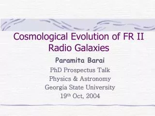
Modeling the Power Evolution of Classical Double Radio Galaxies over Cosmological Scales Dissertation Talk Paramita Barai Dept. of Physics & Astronomy Georgia State University AAS 207th Meeting – Washington, DC 9 January 2006
Motivation • To probe impact of Radio Galaxies (RGs) on the cosmological history of universe • Expanding RGs affected galaxy formation & evolution during the quasar era (1.5 < z < 3) • Trigger star formation Rees – 1989; Gopal-Krishna & Wiita – 2001 • Spread metals and magnetic field into IGM • How much volume of the Relevant Universe (baryonic filaments only) do radio lobes occupy? • Aim: Model individual & cosmological evolution of RGs P. Barai, GSU
Procedures • Semi-analytical models for RG dynamics & power evolution • Compare model predictions with observations • Extensive Statistical test quantifying the success of a model in predicting RG evolution • Choose best model, estimate physical implications Compare model predictions with observations • Virtual (pseudo) Radio Surveys -- Monte Carlo Simulations P. Barai, GSU
Dynamics: Kaiser & Alexander 1997, MNRAS, 286, 215 Power: KDA: Kaiser, Dennett-Thorpe & Alexander 1997, MNRAS, 292, 723 BRW: Blundell, Rawlings & Willott 1999, AJ, 117, 677 MK: Manolakou & Kirk 2002, A&A, 391, 127 K2000: Kaiser 2000, A&A, 362, 447 BRW-modified: Vary hotspot size MK-modified: Vary hotspot size Observables: z, P, D, Low freq. -- 151 MHz: isotropic lobe emission, negligible Doppler boosting Flux-limited, complete radio surveys from Cambridge catalogs: 3CRR 6CE 7CRS Models & Observations P. Barai, GSU
Radio Sky Simulation (BRW)via Multi-dimensional Monte Carlo • RG population generated from early z • Random distribution functions in z, jet power (Q0), age (tage) • Each source’s P, D evolved according to model • At tage, find what flux reaches earth now (from redshift z) • If flux > survey limit, then RG is detected • Populations for 3C, 6C and 7C surveys from same ensemble by its size in ratio to the sky area of each survey • Ensemble size 106 – 107 50-200 detected in virtual surveys
tbir, tage, (zobs), Q0 For each source Sources born every 106 years – from z = 10 tbir TMaxAge = 500 Myr Sources distributed uniformly within comoving cosmological volume tage Jet power distribution if, Qmin < Q0 < Qmax Qmin = 5 1037 W Qmax = 5 1042 W x = 2.6 Redshift distribution z0 = 2.2 z0 = 0.6 Initial RG Population Generation P. Barai, GSU
Radio Luminosity Function (Willott et. al. 2001) P. Barai, GSU
Ambient medium power-law density profile BRW & MK 0 = 1.6710–23 kg m–3 = 1.5 a0 = 10 kpc KDA 0 = 7.210–22 kg m–3 = 1.9 a0 = 2 kpc Size / Total separation between hotspots t : Age of source Q0 : Power of each jet Radio Galaxy Dynamical Evolution P. Barai, GSU
Cylindrical jets move out & accelerate particles (e–' s) at termination shocks Transport of relativistic particles (e– 's) from head to lobe, where they emit (in radio) via synchrotron mechanism Power Losses: Adiabatic loss (as source expands) Inverse Compton scattering off CMB photons Synchrotron radiation BUT key aspects of the models are different Each model ~ 10 parameters Results sensitive to 4–5 of them Energy distribution KDA, MK: Single power-law BRW: break frequencies Adiabatic loss KDA: h.s. pressure with t BRW: Constant h.s. size MK: Ad. losses in head compensated (by some turbulent re-acceleration process) during transport Shared Physics & Variations
Kolmogorov – Smirnov (K–S) test: Find probability, P(K-S) that the quantities of model and observation are drawn from same cumulative distribution population Add the P’s for P, D, z, for the 3 surveys in ratio of the square root of the number detected in a survey: P[P, D, z], P[P, 2D, z] Statistics from several runs (with different initial random seeds) considered for each parameter variation Varied many parameters for each model to possible alternative values Most significant improvement with: x = 3.0 TMaxAge = 150 Myr (KDA & MK) = 250 Myr (BRW) Statistical Test P. Barai, GSU
Parameters of KDA, BRW, MK Models Giving Best Results P. Barai, GSU
Results on Original Models • Some models give acceptable fits for P, D, z • No good fit by any model or variations considered so far • Detection number ratio: MK, KDA, BRW • K-S stat values: MK & KDA > BRW • Overall best – MK • Best (least bad) fits model parameters • x=3.0, TMaxAge = 150, 250 Myr KDA, BRW: • Less dense ambient medium • More efficient acceleration and injection from h.s. to lobes MK: • Contribution from particles of higher & lower energies
Kaiser (2000) proposed modification to KDA: Different ratio of hotspot to lobe pressure I have produced modifications to both BRW and MK: Hot spot size grows as source ages rhs vs. D data Jeyakumar & Saikia 2000, MNRAS, 311, 397 Quadratic fit gave least 2 K2000: too flat P -D tracks, worse statistics P[P, D, z]=0.282, P[P, 2D, z]=0.562 BRW-modified: better K-S stats after introducing growing hotspot size Mean P[P, D, z] = 1.927 Mean P[P, 2D, z] = 2.273 MK-modified: results comparable to or worse than MK default P[P, D, z]=1.72, P[P, 2D, z]=2.34 Modifications to the Models
Environment density becomes constant after ISM-IGM boundary Redshift evolution of ambient medium density 0, a0, changes with z Incorporate Doppler-boosted core and jet emission to predict total power emitted See if same models can be used to match larger, deeper radio survey catalogs: NVSS, WENSS, FIRST Poster: session 25, Kimball et al. Adopt best model Compute the volume fraction of the relevant universe filled by radio lobes Discuss cosmological impact of expanding RGs Current Work & Future Plans
Summary • Made quantitative comparisons between models of RG evolution using our extensive simulations and K-S test based statistical analysis • Some published models give acceptable fits to P, D, z of radio surveys 3C, 6C, 7C • Modified models can give improved fits and will be extended to deeper radio surveys P. Barai, GSU
References • Blundell K.M., Rawlings S. & Willott C.J. 1999, AJ, 117, 677 (BRW) • Gopal-Krishna & Wiita P.J. 2001, ApJ, 560, L115 • Jeyakumar S. & Saikia D.J. 2000, MNRAS, 311, 397 • Kaiser C.R. & Alexander P. 1997, MNRAS, 286, 215 • Kaiser C.R., Dennett-Thorpe J. & Alexander P. 1997, MNRAS, 292, 723 (KDA) • Kaiser C.R. 2000, A&A, 362, 447 (K2000) • Manolakou K. & Kirk J.G. 2002, A&A, 391, 127 (MK) • Rees M.J. 1989, MNRAS, 239, 1P P. Barai, GSU