Clustering with k-means Lantz Ch 9

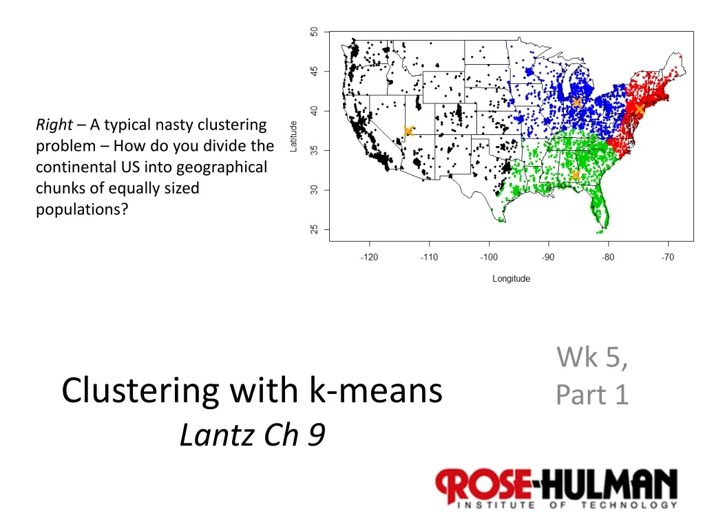
1. Right – A typical nasty clustering problem – How do you divide the continental US into geographical chunks of equally sized populations? Clustering with k-meansLantz Ch 9 Wk 5, Part 1

2. Early warning – stereotypes! • This is supplying data to justify grouping people or things in ways you’re already set on.

3. E.g., race and intelligence • E.g., In his later life, Nobel prize winner William Shockley infamously used grouping to show statistically some racial groups had lower average IQ’s. • But he ignored the fact that IQ also had geographical variations, for example.

4. Generally unsupervised • Clustering usually is exploratory. • Like, what sales are associated with other sales. • There is an end goal. • Like, how can we reorganize product promotions to create more add-on sales.

5. Often, we want a simpler picture • What are the natural groupings for a large number of features? • We may not even have names for our groups, at the start. • We figure these out as we go. • Thinking of groups and possible actions for them – an interactive thought process.

6. Clustering creates new data • We invent concepts from it. • The groups may, initially, be without names. • Madeleine L’Engle would be horrified. • Plot of “A Wrinkle in Time” was that “dark” things had no names – this needed to be fixed! Wait, wait – I dub thee a “tesseract”!

7. Lantz’s example – setting up networking at a conference • There are math people, and • There are computer science people:

8. Can machine learning cluster these for us, to help identify groups? • We have to supply the name tags, of course:

9. The k-means algorithm

10. Use distance to identify clusters • Choose initial cluster centers. • How many? User guesses a number. • Then, how far are other points from these?

11. This leads to defining initial boundaries • Use our old friends, the convex polygons, etc. • Slightly simpler, if few categories: • But, how do we know this division is optimal? • We don’t!

12. Change the initial cluster centers… • Calculate the “centroid” (central point) of each group. • Then re-decide what other points are closest to each centroid.

13. Additional cycles of updates • Changing the centroids, then changing what’s closest to them, can be done several times. Final result?

14. But – How many clusters? • More more clusters  more homogeneity in the features • Which may be based partly on noise! • Look for “knee bend” as a likely point to stop increasing the number.

15. Lantz’s example – Teen market segments > str(teens) 'data.frame': 30000 obs. of 40 variables: $ gradyear : int 2006 2006 2006 2006 2006 2006 2006 2006 2006 2006 ... $ gender : Factor w/ 2 levels "F","M": 2 1 2 1 NA 1 1 2 1 1 ... $ age : num 19 18.8 18.3 18.9 19 ... $ friends : int 7 0 69 0 10 142 72 17 52 39 ... $ basketball : int 0 0 0 0 0 0 0 0 0 0 ... $ football : int 0 1 1 0 0 0 0 0 0 0 ... $ soccer : int 0 0 0 0 0 0 0 0 0 0 ... $ softball : int 0 0 0 0 0 0 0 1 0 0 ... $ volleyball : int 0 0 0 0 0 0 0 0 0 0 ... $ swimming : int 0 0 0 0 0 0 0 0 0 0 ... $ cheerleading: int 0 0 0 0 0 0 0 0 0 0 ... $ baseball : int 0 0 0 0 0 0 0 0 0 0 ... $ tennis : int 0 0 0 0 0 0 0 0 0 0 ... $ sports : int 0 0 0 0 0 0 0 0 0 0 ... $ cute : int 0 1 0 1 0 0 0 0 0 1 ... $ sex : int 0 0 0 0 1 1 0 2 0 0 ... $ sexy : int 0 0 0 0 0 0 0 1 0 0 ... $ hot : int 0 0 0 0 0 0 0 0 0 1 ... $ kissed : int 0 0 0 0 5 0 0 0 0 0 ... $ dance : int 1 0 0 0 1 0 0 0 0 0 ... $ band : int 0 0 2 0 1 0 1 0 0 0 ... $ marching : int 0 0 0 0 0 1 1 0 0 0 ... $ music : int 0 2 1 0 3 2 0 1 0 1 ... $ rock : int 0 2 0 1 0 0 0 1 0 1 ... $ god : int 0 1 0 0 1 0 0 0 0 6 ... $ church : int 0 0 0 0 0 0 0 0 0 0 ... $ jesus : int 0 0 0 0 0 0 0 0 0 2 ... $ bible : int 0 0 0 0 0 0 0 0 0 0 ... $ hair : int 0 6 0 0 1 0 0 0 0 1 ... $ dress : int 0 4 0 0 0 1 0 0 0 0 ... $ blonde : int 0 0 0 0 0 0 0 0 0 0 ... $ mall : int 0 1 0 0 0 0 2 0 0 0 ... $ shopping : int 0 0 0 0 2 1 0 0 0 1 ... $ clothes : int 0 0 0 0 0 0 0 0 0 0 ... $ hollister : int 0 0 0 0 0 0 2 0 0 0 ... $ abercrombie : int 0 0 0 0 0 0 0 0 0 0 ... $ die : int 0 0 0 0 0 0 0 0 0 0 ... $ death : int 0 0 1 0 0 0 0 0 0 0 ... $ drunk : int 0 0 0 0 1 1 0 0 0 0 ... $ drugs : int 0 0 0 0 1 0 0 0 0 0 ...

16. Need to understand / fix “NA’s” > table(teens$gender, useNA = "ifany”) F M <NA> 22054 5222 2724 > summary(teens$age) Min. 1st Qu. Median Mean 3rd Qu. Max. NA's 3.086 16.310 17.290 17.990 18.260 106.900 5086

17. For marketing we want “interest” clusters for these teens > interests <- teens[5:40] > interests_z <- as.data.frame(lapply(interests, scale)) > teen_clusters <- kmeans(interests_z, 5) > teen_clusters$size [1] 1061 5008 720 22562 649 Put them on a uniform scale! One cluster is lots bigger!

18. We can characterize these clusters • Look at their centroids. • Where are the strong + and – values? We then provide the stereotypes!

19. Improving on these results? • Go back and look at the data, given our new cluster knowledge: > teens[1:5, c("cluster", "gender", "age", "friends")] cluster gender age friends 1 4 M 18.982 7 2 2 F 18.801 0 3 4 M 18.335 69 4 4 F 18.875 0 5 1 <NA> 18.995 10

20. Aggregate data make sense? > aggregate(data = teens, friends ~ cluster, mean) cluster friends 1 1 30.68143 2 2 38.69269 3 3 35.77917 4 4 27.93932 5 5 35.33128