Download
1 / 34
340 likes | 357 Views
Explore various numerical methods for solving nonlinear equations, including Bisection, Newton's, Secant methods, and more. Understand algorithms, assumptions, and implementation in Matlab.

E N D
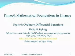
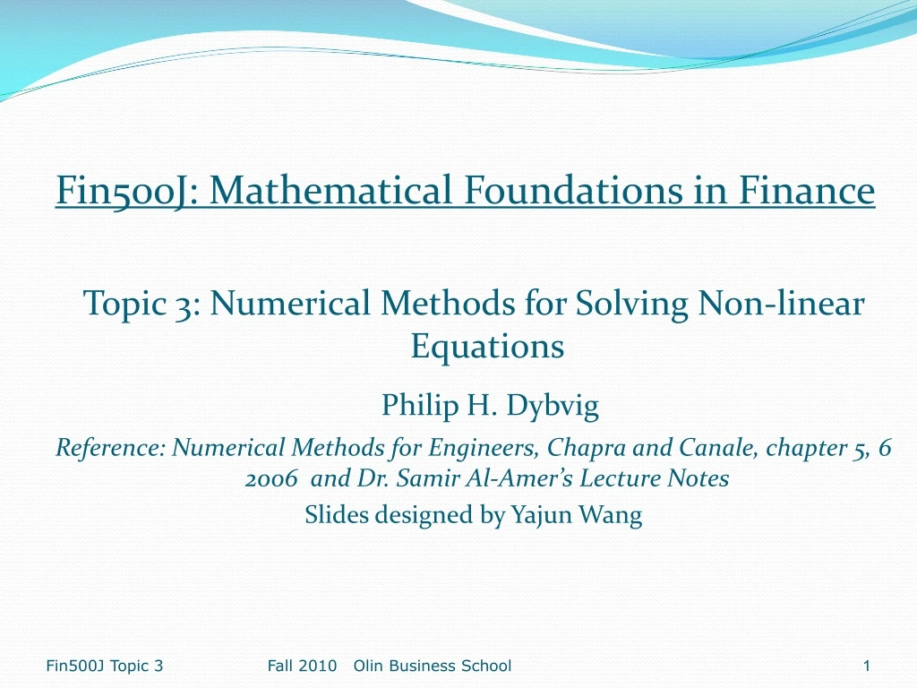
Fin500J: Mathematical Foundations in Finance Topic 3: Numerical Methods for Solving Non-linear Equations Philip H. Dybvig Reference: Numerical Methods for Engineers, Chapra and Canale, chapter 5, 6 2006 and Dr. Samir Al-Amer’s Lecture Notes Slides designed by Yajun Wang Fall 2010 Olin Business School
Solution Methods Several ways to solve nonlinear equations are possible. • Analytical Solutions • possible for special equations only • Graphical Illustration • Useful for providing initial guesses for other methods • Numerical Solutions • Open methods • Bracketing methods Fall 2010 Olin Business School
Solution Methods:Analytical Solutions Analytical solutions are available for special equations only. Fall 2010 Olin Business School
Graphical Illustration • Graphical illustration are useful to provide an initial guess to be used by other methods Root 2 1 1 2 Fall 2010 Olin Business School
Bracketing/Open Methods • In bracketing methods, the method starts with an interval that contains the root and a procedure is used to obtain a smaller interval containing the root. • Examples of bracketing methods : Bisection method • In the open methods, the method starts with one or more initial guess points. In each iteration a new guess of the root is obtained. Fall 2010 Olin Business School
Solution Methods Many methods are available to solve nonlinear equations • Bisection Method • Newton’s Method • Secant Method • False position Method • Muller’s Method • Bairstow’s Method • Fixed point iterations • ………. These will be covered. Fall 2010 Olin Business School
Bisection Method • The Bisection method is one of the simplest methods to find a zero of a nonlinear function. • To use the Bisection method, one needs an initial interval that is known to contain a zero of the function. • The method systematically reduces the interval. It does this by dividing the interval into two equal parts, performs a simple test and based on the result of the test half of the interval is thrown away. • The procedure is repeated until the desired interval size is obtained. Fall 2010 Olin Business School
Intermediate Value Theorem • Let f(x) be defined on the interval [a,b], • Intermediate value theorem: if a function is continuous and f(a) and f(b) have different signs then the function has at least one zero in the interval [a,b] f(a) a b f(b) Fall 2010 Olin Business School
Bisection Algorithm Assumptions: • f(x) is continuous on [a,b] • f(a) f(b) < 0 Algorithm: Loop 1. Compute the mid point c=(a+b)/2 2. Evaluate f(c ) 3. If f(a) f(c) < 0 then new interval [a, c] If f(a) f( c) > 0 then new interval [c, b] End loop f(a) c b a f(b) Fall 2010 Olin Business School
Bisection Method Assumptions: Given an interval [a,b] f(x) is continuous on [a,b] f(a) and f(b) have opposite signs. These assumptions ensures the existence of at least one zero in the interval [a,b] and the bisection method can be used to obtain a smaller interval that contains the zero. Fall 2010 Olin Business School
Bisection Method b0 a0 a1 a2 Fall 2010 Olin Business School
Flow chart of Bisection Method Start: Given a,b and ε u = f(a) ; v = f(b) c = (a+b) /2 ; w = f(c) no yes is (b-a)/2 <ε is u w <0 no Stop yes b=c; v= w a=c; u= w Fall 2010 Olin Business School
Example: Answer: Fall 2010 Olin Business School
Stopping Criteria Two common stopping criteria • Stop after a fixed number of iterations • Stop when Fall 2010 Olin Business School
Example • Use Bisection method to find a root of the equation x = cos (x) with (b-a)/2n+1<0.02 (assume the initial interval [0.5,0.9]) Question 1: What is f (x) ? Question 2: Are the assumptions satisfied ? Fall 2010 Olin Business School
Bisection MethodInitial Interval f(a)=-0.3776 f(b) =0.2784 a =0.5 c= 0.7 b= 0.9 Fall 2010 Olin Business School
-0.3776 -0.06480.2784 (0.9-0.7)/2 = 0.1 0.5 0.7 0.9 -0.06480.1033 0.2784 (0.8-0.7)/2 = 0.05 0.7 0.8 0.9 Fall 2010 Olin Business School
-0.06480.0183 0.1033 (0.75-0.7)/2= 0.025 0.7 0.75 0.8 -0.0648 -0.02350.0183 (0.75-0.725)/2= .0125 0.70 0.725 0.75 Fall 2010 Olin Business School
Summary • Initial interval containing the root [0.5,0.9] • After 4 iterations • Interval containing the root [0.725 ,0.75] • Best estimate of the root is 0.7375 • | Error | < 0.0125 Fall 2010 Olin Business School
Bisection Method Programming in Matlab c = 0.7000 fc = -0.0648 c = 0.8000 fc = 0.1033 c = 0.7500 fc = 0.0183 c = 0.7250 fc = -0.0235 a=.5; b=.9; u=a-cos(a); v= b-cos(b); for i=1:5 c=(a+b)/2 fc=c-cos(c) if u*fc<0 b=c ; v=fc; else a=c; u=fc; end end Fall 2010 Olin Business School
Newton-Raphson Method (also known as Newton’s Method) Given an initial guess of the root x0 , Newton-Raphson method uses information about the function and its derivative at that point to find a better guess of the root. Assumptions: • f (x) is continuous and first derivative is known • An initial guess x0 such that f ’(x0) ≠0 is given Fall 2010 Olin Business School
Newton’s Method Xi+1 Xi Fall 2010 Olin Business School
Example FN.m FNP.m Fall 2010 Olin Business School
Results • X = 0.5379 FNX =0.0461 • X =0.5670 FNX =2.4495e-004 • X = 0.5671 FNX =6.9278e-009 Fall 2010 Olin Business School
Secant Method Fall 2010 Olin Business School
Secant Method Fall 2010 Olin Business School
Example Fall 2010 Olin Business School
Example Fall 2010 Olin Business School
Results Xi = -1 FXi =1 Xi =-1.1000 FXi =0.0585 Xi =-1.1062 FXi =-0.0102 Xi =-1.1053 FXi =8.1695e-005 Xi = -1.1053 FXi =1.1276e-007 Fall 2010 Olin Business School
Summary Fall 2010 Olin Business School
Solving Non-linear Equation using Matlab • Example (i): find a root of f(x)=x-cos x, in [0,1] • >> f=@(x) x-cos(x); • >> fzero(f,[0,1]) • ans = • 0.7391 • Example (ii): find a root of f(x)=e-x-x using the initial point x=1 • >> f=@(x) exp(-x)-x; • >> fzero(f,1) • ans = • 0.5671 Fall 2010 Olin Business School
Solving Non-linear Equation using Matlab • Example (iii): find a root of f(x)=x5+x3+3 around -1 • >> f=@(x) x^5+x^3+3; • >> fzero(f,-1) • ans = • -1.1053 • Because this function is a polynomial, we can find other roots • >> roots([1 0 1 0 0 3]) • ans = • 0.8719 + 0.8063i • 0.8719 - 0.8063i • -0.3192 + 1.3501i • -0.3192 - 1.3501i • -1.1053 Fall 2010 Olin Business School
Use fzero Solver in Matlab • >>optimtool • For example: • want to find a root around -1 for x5+x3+3=0 • The algorithm of fzero uses a combination of bisection, secant, etc. Fall 2010 Olin Business School