Download
1 / 86
860 likes | 875 Views
Explore efficient search algorithms for solving decision problems through state space navigation. Learn about various algorithms like Breadth-First, Depth-First Search, and more with examples and limitations. Understand the concepts of goal-based and utility-based search agents. Delve into problem formulations, algorithm application, and state space representation using search graphs and trees. Enhance your problem-solving skills in different environments with this comprehensive guide.

E N D
Agents Solving Problems byEnvironment State Space Search Jacques Robin
Outline • Search Agent • Formulating Decision Problems as Navigating State Space to Find Goal State • Generic Search Algorithm • Specific Algorithms • Breadth-First Search • Uniform Cost Search • Depth-First Search • Backtracking Search • Iterative Deepening Search • Bi-Directional Search • Comparative Table • Limitations and Difficulties • Repeated States • Partial Information
Search Agents • Generic decision problem to be solved by an agent: • Among all possible action sequences that I can execute, • which ones will result in changing the environment from its current state, • to another state that matches my goal? • Additional optimization problem: • Among those action sequences that will change the environment from its current state to a goal state • which one can be executed at minimum cost? • or which one leads to a state with maximum utility? • Search agent solves this decision problem by a generate and test approach: • Given the environment model, • generate one by one (all) the possible states (the state space) of the environment reachable through all possible action sequences from the current state, • test each generated state to determine whether it satisfies the goal or maximize utility • Navigation metaphor: • The order of state generation is viewed as navigating the entire environment state space
Off-Line Goal-Based Search Agent Environment Agent P Percept Interpretation: Environment Initialization Sensors Action Sequence EffectPrediction: Search Algorithm E: EnvironmentModel goalTest():Boolean S: ActionSequence S Effectors
Off-Line Utility-Based Search Agent Environment Agent P Percept Interpretation: Environment Initialization Sensors Action Sequence EffectPrediction: Search Algorithm E: EnvironmentModel utility():Number S: ActionSequence S Effectors
On-Line Goal-Based Search Agent Environment Agent P Percept Interpretation: Environment Update Sensors Single Action EffectPrediction: Search Algorithm E: EnvironmentModel goalTest():Boolean A Effectors
On-Line Utility-Based Search Agent Environment Agent P Percept Interpretation: Environment Update Sensors Single Action EffectPrediction: Search Algorithm E: EnvironmentModel utility():Number A Effectors
Q Q Q Q Q Q Q Q Q Q Q Q Q Q Q Q Q Q Q Q Move Queen Move Queen Q Q Problem Algorithm Insert Queen Insert Queen Insert Queen Insert Queen Navigation Metaphor Example of Applying Navigation Metaphorto Arbitrary Decision Problem • N-Queens problem: how to arrange n queens on a NxN chess board in a pacific configuration where no queen can attack another? • Full-State Formulation: local navigation in thefull-State Space • Partial-State Formulation: global navigation in partial-State Space
disjoint, complete overlapping, complete disjoint, complete disjoint, complete Full-State Space Search Problem initState: FullState typicalState: FullState action: ModifyStateAction Partial-State Space Search Problem initialState: EmptyState typicalState: PartialState goalState: FullState action: RefineStateAction Goal-Satisfaction Search Problem Test: GoalSatisfactionTest Optimization Search Problem Test: utilityMaximizationTest On-Line Search Problem solution: Action Path Finding Search Problem solution: Path State Finding Search Problem solution: State Off-Line Search Problem solution: Sequence(Action) disjoint, incomplete Sensorless Search Problem sensor: MissingSensor action: DeterministicAction envModel: NonMissing Contingency Search Problem sensor: PartialSensor action: DeterministicAction envModel: CompleteEnvModel Exploration Search Problem sensor: PartialSensor action: DeterministicAction envModel: Missing Fully Informed Search Problem sensor: CompletePerfectSensor action: DeterministicAction envtModel: CompleteEnvModel Search Problem Taxonomy Search Problem
Search Graphs and SearchTrees • The state space can be represented as a search graph or a search tree • Each search graph or tree node represents an environment state • Each search graph or tree arc represents an action changing the environment from its source node to its target node • Each node or arc can be associated to a utility or cost • Each path from one node to another represents an action sequence • In search tree, the root node represents the initial state and some leaves represent goal states • The problem of navigating the state space then becomes one of generating and maintaining a search graph or tree until a solution node or path is generated • The problem search graph or tree: • An abstract concept that contains one node for each possible environment state • Can be infinite • The algorithm search graph or tree: • A concrete data structure • A subset of the problem search graph or tree that contains only the nodes generated and maintained (i.e., explored) at the current point during the algorithm execution (always finite) • Problem search graph or tree branching factor: average number of actions available to the agent in each state • Algorithm effective branching factor: average number of nodes effectively generated as successors of each node during search
c d c c,d c d c c,d c d c,d c,d d c d c c,d d c,d d d c d d c,d c d c,d d c d c c c,d d d c c,d d c,d d c c c,d d d d c,d c,d c,d d d d d c,d d d c c,d d d c d c,d d c c,d d d c d d c,d c d d c d c,d d d c,d c,d c,d c,d d Search Graph and Tree Examples:Vacuum Cleaner World u u u u s s s u c u d u d u d s s c s d s s d d d d u s d u d u s d s u s d
Search Methods • Searching the entire space of the action sequence reachable environment states is called exhaustive search, systematic search, blind search or uninformed search • Searching a restricted subset of that state space based on knowledge about the specific characteristics of the problem or problem class is called partial search • A heuristic is an insight or approximate knowledge about a problem class or problem class family on which a search algorithm can rely to improve its run time and/or space requirement • An ordering heuristic defines: • In which order to generate the problem search tree nodes, • Where to go next while navigating the state space (to get closer faster to a solution point) • A pruning heuristic defines: • Which branches of the problem search tree to avoid generating alltogether, • What subspaces of the state space not to explore (for they cannot or are very unlikely to contain a solution point) • Non-heuristic, exhaustive search is not scalable to large problem instances (worst-case exponential in time and/or space) • Heuristic, partial search offers no warrantee to find a solution if one exist, or to find the best solution if several exists.
Formulating a Agent Decision Problemas a Search Problem • Define abstract format of ageneric environment state, ex., a class C • Define the initial state, ex., a specific object of class C • Define the successor operation: • Takes as input a state or state set S and an action A • Returns the state or state set R resulting from the agent executing A in S • Together, these 3 elements constitute an intentional representation of the state space • The search algorithm transforms this intentional representation into an extensional one, by repeatedly applying the successor operation starting from the initial state • Define a boolean operation testing whether a state is a goal, ex., a method of C • For optimization problems: additionally define a operation that returns the cost or utility of an action or state
Problem Formulation Most Crucial Factorof Search Efficiency • Problem formulation is more crucial than choice of search algorithm or choice of heuristics to make an agent decision problem effectively solvable by state space search • 8-queens problem formulation 1: • Initial state: empty board • Action: pick column and line of one queen • Branching factor: 64 • State-space: ~648 • 8-queens problem formulation 2: • Initial state: empty board • Action: pre-assign one column per queen, pick only line in pre-assigned column • Branching factor: 8 • State-space: ~88
fringe Generic Exhaustive Search Algorithm • Initialize the fringe to the root node representing the initial state • Until goal node found in fringe, repeat: • Choose one node from fringe to expand by calling its successor operation • Extend the current fringe with the nodes generated by this successor operation • If optimization problem, update path cost or utility value • Return goal node or path from root node to goal node Specific algorithms differ in terms of the order in which they respectively expand the fringe nodes Arad Sibiu Timisoara Zenrid Arad Fagaras Oradea R.Vilcea Arad Lugoj Arad Oradea
Generic Exhaustive Search Algorithm • Initialize the fringe to the root node representing the initial state • Until goal node found in fringe, repeat: • Choose one node from fringe to expand by calling its successor operation • Extend the current fringe with the nodes generated by this successor operation • If optimization problem, update path cost or utility value • Return goal node or path from root node to goal node Specific algorithms differ in terms of the order in which they respectively expand the fringe nodes Arad fringe Sibiu Timisoara Zenrid Arad Fagaras Oradea R.Vilcea Arad Lugoj Arad Oradea
Generic Exhaustive Search Algorithm • Initialize the fringe to the root node representing the initial state • Until goal node found in fringe, repeat: • Choose one node from fringe to expand by calling its successor operation • Extend the current fringe with the nodes generated by this successor operation • If optimization problem, update path cost or utility value • Return goal node or path from root node to goal node Specific algorithms differ in terms of the order in which they respectively expand the fringe nodes Arad open-list Sibiu Timisoara Zenrid fringe Arad Fagaras Oradea R.Vilcea Arad Lugoj Arad Oradea
Search Algorithms Characteristics and Performance • Complete: guaranteed to find a solution if one exists • Optimal (for optimization problem): guaranteed to find the best (highest utility or lowest cost) solution if one exists • Input parameters to complexity metrics: • b = problem search tree branching factor • d = depth of highest solution (or best solution for optimization problems) in problem search tree • m = problem search tree depth (can be infinite) • Complexity metrics of algorithms: • TimeComplexity(b,d,m) = number of expanded nodes • SpaceComplexity(b,d,m) = maximum number of nodes needed in memory at one point during the execution of the algorithm
Exhaustive Search Algorithms • Breadth-First: Expand first most shallow node from fringe • Uniform Cost: Expand first node from fringe of lowest cost (or highest utility) path from the root node • Depth-First: Expand first deepest node from fringe • Backtracking: Depth first variant with fringe limited to a single node • Depth-Limited: Depth-first stopping at depth limit N. • Iterative Deepening: Sequence of depth limited search at increasing depth • Bi-directional: • Parallel search from initial state and from goal state • Solution found when the two paths under construction intersect
Breadth-First Search Fringe A B C D E F G H I J K L M N O
Breadth-First Search Fringe A Expanded B C D E F G H I J K L M N O
Breadth-First Search Fringe A Expanded B C D E F G H I J K L M N O
Breadth-First Search Fringe A Expanded B C D E F G H I J K L M N O
Breadth-First Search Fringe A Expanded B C D E F G H I J K L M N O
Breadth-First Search Fringe A Expanded B C D E F G H I J K L M N O
Breadth-First Search Fringe A Expanded B C D E F G H I J K L M N O
Breadth-First Search Fringe A Expanded B C D E F G H I J K L M N O
A A A A B C D B C D B C D 1 15 5 15 5 15 EB EB Ec 11 11 10 Uniform Cost Search B 10 1 5 5 Problem Graph: C E A 15 5 D
Depth-First Search A B C D E F G H I J K L M N O
Depth-First Search A B C D E F G H I J K L M N O
Depth-First Search A B C D E F G H I J K L M N O
Depth-First Search A B C D E F G H I J K L M N O
Depth-First Search A B C D E F G H I J K L M N O
Depth-First Search A B C D E F G H I J K L M N O
Depth-First Search A B C D E F G H I J K L M N O
Depth-First Search A B C D E F G H I J K L M N O
Depth-First Search A B C D E F G H I J K L M N O
Backtracking Search A B C D E F G H I J K L M N O
Backtracking Search A B C D E F G H I J K L M N O
Depth-First Search A B C D E F G H I J K L M N O
Backtracking Search A B C D E F G H I J K L M N O
Backtracking Search A B C D E F G I J K L M N O
Backtracking Search A B C E F G J K L M N O
Backtracking Search A B C E F G J K L M N O
Backtracking Search A B C E F G K L M N O
Backtracking Search A C F G L M N O
L = 0 A L = 1 A A A A B C B C B C L = 2 A A A A B C B C B C D E D E A A A A B C B C B C B C D E D E D E D E D E D E D E Iterative Deepening A
Bi-Directional Search • Two parallel searches: one from the current state and one from the goal state • When they reach a common node: a path from current to goal has been found • Time complexity halved: O(bd/2) + O(bd/2) = O(bd/2) << O(bd) • But not alwayspossible: • Irreversibleactions • Large numberof intentionallyspecifiedgoal states
Comparing Search Algorithms • C* = cost of optimal solution • a actions(agent), cost(a) e