Download
1 / 37
370 likes | 701 Views
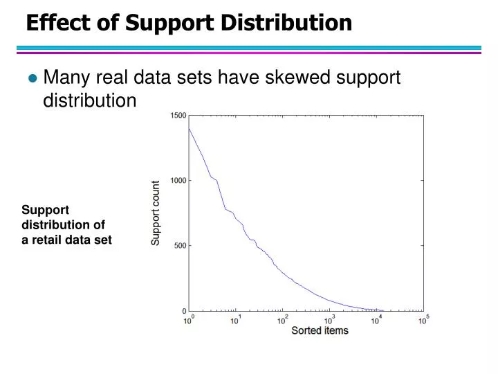
Effect of Support Distribution. Many real data sets have skewed support distribution. Support distribution of a retail data set. Effect of Support Distribution. How to set the appropriate minsup threshold?

E N D
Effect of Support Distribution • Many real data sets have skewed support distribution Support distribution of a retail data set
Effect of Support Distribution • How to set the appropriate minsup threshold? • If minsup is set too high, we could miss itemsets involving interesting rare items (e.g., expensive products) • If minsup is set too low, it is computationally expensive and the number of itemsets is very large • Using a single minimum support threshold may not be effective
Multiple Minimum Support • How to apply multiple minimum supports? • MS(i): minimum support for item i • e.g.: MS(Milk)=5%, MS(Coke) = 3%, MS(Broccoli)=0.1%, MS(Salmon)=0.5% • MS({Milk, Broccoli}) = min (MS(Milk), MS(Broccoli)) = 0.1% • Challenge: Support is no longer anti-monotone • Suppose: Support(Milk, Coke) = 1.5% and Support(Milk, Coke, Broccoli) = 0.5% • {Milk,Coke} is infrequent but {Milk,Coke,Broccoli} is frequent
Multiple Minimum Support (Liu 1999) • Order the items according to their minimum support (in ascending order) • e.g.: MS(Milk)=5%, MS(Coke) = 3%, MS(Broccoli)=0.1%, MS(Salmon)=0.5% • Ordering: Broccoli, Salmon, Coke, Milk • Need to modify Apriori such that: • L1 : set of frequent items • F1 : set of items whose support is MS(1) where MS(1) is mini( MS(i) ) • C2 : candidate itemsets of size 2 is generated from F1instead of L1
Multiple Minimum Support (Liu 1999) • Modifications to Apriori: • In traditional Apriori, • A candidate (k+1)-itemset is generated by merging two frequent itemsets of size k • The candidate is pruned if it contains any infrequent subsets of size k • Pruning step has to be modified: • Prune only if subset contains the first item • e.g.: Candidate={Broccoli, Coke, Milk} (ordered according to minimum support) • {Broccoli, Coke} and {Broccoli, Milk} are frequent but {Coke, Milk} is infrequent • Candidate is not pruned because {Coke,Milk} does not contain the first item, i.e., Broccoli.
Mining Various Kinds of Association Rules • Mining multilevel association • Miming multidimensional association • Mining quantitative association • Mining interesting correlation patterns
uniform support reduced support Level 1 min_sup = 5% Milk [support = 10%] Level 1 min_sup = 5% Level 2 min_sup = 5% 2% Milk [support = 6%] Skim Milk [support = 4%] Level 2 min_sup = 3% Mining Multiple-Level Association Rules • Items often form hierarchies • Flexible support settings • Items at the lower level are expected to have lower support • Exploration of shared multi-level mining (Agrawal & Srikant@VLB’95, Han & Fu@VLDB’95)
Multi-level Association: Redundancy Filtering • Some rules may be redundant due to “ancestor” relationships between items. • Example • milk wheat bread [support = 8%, confidence = 70%] • 2% milk wheat bread [support = 2%, confidence = 72%] • We say the first rule is an ancestor of the second rule. • A rule is redundant if its support is close to the “expected” value, based on the rule’s ancestor.
Mining Multi-Dimensional Association • Single-dimensional rules: buys(X, “milk”) buys(X, “bread”) • Multi-dimensional rules: 2 dimensions or predicates • Inter-dimension assoc. rules (no repeated predicates) age(X,”19-25”) occupation(X,“student”) buys(X, “coke”) • hybrid-dimension assoc. rules (repeated predicates) age(X,”19-25”) buys(X, “popcorn”) buys(X, “coke”) • Categorical Attributes: finite number of possible values, no ordering among values—data cube approach • Quantitative Attributes: numeric, implicit ordering among values—discretization, clustering, and gradient approaches
Mining Quantitative Associations • Techniques can be categorized by how numerical attributes, such as age or salary are treated • Static discretization based on predefined concept hierarchies (data cube methods) • Dynamic discretization based on data distribution (quantitative rules, e.g., Agrawal & Srikant@SIGMOD96) • Clustering: Distance-based association (e.g., Yang & Miller@SIGMOD97) • one dimensional clustering then association • Deviation: (such as Aumann and Lindell@KDD99) Sex = female => Wage: mean=$7/hr (overall mean = $9)
() (age) (income) (buys) (age, income) (age,buys) (income,buys) (age,income,buys) Static Discretization of Quantitative Attributes • Discretized prior to mining using concept hierarchy. • Numeric values are replaced by ranges. • In relational database, finding all frequent k-predicate sets will require k or k+1 table scans. • Data cube is well suited for mining. • The cells of an n-dimensional cuboid correspond to the predicate sets. • Mining from data cubescan be much faster.
Quantitative Association Rules • Proposed by Lent, Swami and Widom ICDE’97 • Numeric attributes are dynamically discretized • Such that the confidence or compactness of the rules mined is maximized • 2-D quantitative association rules: Aquan1 Aquan2 Acat • Cluster adjacent association rules to form general rules using a 2-D grid • Example age(X,”34-35”) income(X,”30-50K”) buys(X,”high resolution TV”)
Mining Other Interesting Patterns • Flexible support constraints (Wang et al. @ VLDB’02) • Some items (e.g., diamond) may occur rarely but are valuable • Customized supmin specification and application • Top-K closed frequent patterns (Han, et al. @ ICDM’02) • Hard to specify supmin, but top-kwith lengthmin is more desirable • Dynamically raise supmin in FP-tree construction and mining, and select most promising path to mine
Pattern Evaluation • Association rule algorithms tend to produce too many rules • many of them are uninteresting or redundant • Redundant if {A,B,C} {D} and {A,B} {D} have same support & confidence • Interestingness measures can be used to prune/rank the derived patterns • In the original formulation of association rules, support & confidence are the only measures used
Interestingness Measures Application of Interestingness Measure
f11: support of X and Yf10: support of X and Yf01: support of X and Yf00: support of X and Y Computing Interestingness Measure • Given a rule X Y, information needed to compute rule interestingness can be obtained from a contingency table Contingency table for X Y Used to define various measures • support, confidence, lift, Gini, J-measure, etc.
Association Rule: Tea Coffee • Confidence= P(Coffee|Tea) = 0.75 • but P(Coffee) = 0.9 • Although confidence is high, rule is misleading • P(Coffee|Tea) = 0.9375 Drawback of Confidence
Statistical Independence • Population of 1000 students • 600 students know how to swim (S) • 700 students know how to bike (B) • 420 students know how to swim and bike (S,B) • P(SB) = 420/1000 = 0.42 • P(S) P(B) = 0.6 0.7 = 0.42 • P(SB) = P(S) P(B) => Statistical independence • P(SB) > P(S) P(B) => Positively correlated • P(SB) < P(S) P(B) => Negatively correlated
Statistical-based Measures • Measures that take into account statistical dependence
Example: Lift/Interest • Association Rule: Tea Coffee • Confidence= P(Coffee|Tea) = 0.75 • but P(Coffee) = 0.9 • Lift = 0.75/0.9= 0.8333 (< 1, therefore is negatively associated)
Drawback of Lift & Interest Statistical independence: If P(X,Y)=P(X)P(Y) => Lift = 1
Interestingness Measure: Correlations (Lift) • play basketball eat cereal [40%, 66.7%] is misleading • The overall % of students eating cereal is 75% > 66.7%. • play basketball not eat cereal [20%, 33.3%] is more accurate, although with lower support and confidence • Measure of dependent/correlated events: lift
Are lift and 2 Good Measures of Correlation? • “Buy walnuts buy milk [1%, 80%]” is misleading • if 85% of customers buy milk • Support and confidence are not good to represent correlations • So many interestingness measures? (Tan, Kumar, Sritastava @KDD’02)
Which Measures Should Be Used? • lift and 2are not good measures for correlations in large transactional DBs • all-conf or coherence could be good measures (Omiecinski@TKDE’03) • Both all-conf and coherence have the downward closure property • Efficient algorithms can be derived for mining (Lee et al. @ICDM’03sub)
There are lots of measures proposed in the literature Some measures are good for certain applications, but not for others What criteria should we use to determine whether a measure is good or bad? What about Apriori-style support based pruning? How does it affect these measures?
Support-based Pruning • Most of the association rule mining algorithms use support measure to prune rules and itemsets • Study effect of support pruning on correlation of itemsets • Generate 10000 random contingency tables • Compute support and pairwise correlation for each table • Apply support-based pruning and examine the tables that are removed
Effect of Support-based Pruning Support-based pruning eliminates mostly negatively correlated itemsets
Effect of Support-based Pruning • Investigate how support-based pruning affects other measures • Steps: • Generate 10000 contingency tables • Rank each table according to the different measures • Compute the pair-wise correlation between the measures
Effect of Support-based Pruning • Without Support Pruning (All Pairs) Scatter Plot between Correlation & Jaccard Measure • Red cells indicate correlation between the pair of measures > 0.85 • 40.14% pairs have correlation > 0.85
Effect of Support-based Pruning • 0.5% support 50% Scatter Plot between Correlation & Jaccard Measure: • 61.45% pairs have correlation > 0.85
Effect of Support-based Pruning • 0.5% support 30% Scatter Plot between Correlation & Jaccard Measure • 76.42% pairs have correlation > 0.85
Subjective Interestingness Measure • Objective measure: • Rank patterns based on statistics computed from data • e.g., 21 measures of association (support, confidence, Laplace, Gini, mutual information, Jaccard, etc). • Subjective measure: • Rank patterns according to user’s interpretation • A pattern is subjectively interesting if it contradicts the expectation of a user (Silberschatz & Tuzhilin) • A pattern is subjectively interesting if it is actionable (Silberschatz & Tuzhilin)
Interestingness via Unexpectedness • Need to model expectation of users (domain knowledge) • Need to combine expectation of users with evidence from data (i.e., extracted patterns) + Pattern expected to be frequent - Pattern expected to be infrequent Pattern found to be frequent Pattern found to be infrequent - + Expected Patterns - + Unexpected Patterns
Interestingness via Unexpectedness • Web Data (Cooley et al 2001) • Domain knowledge in the form of site structure • Given an itemset F = {X1, X2, …, Xk} (Xi : Web pages) • L: number of links connecting the pages • lfactor = L / (k k-1) • cfactor = 1 (if graph is connected), 0 (disconnected graph) • Structure evidence = cfactor lfactor • Usage evidence • Use Dempster-Shafer theory to combine domain knowledge and evidence from data