Download
1 / 11
110 likes | 223 Views
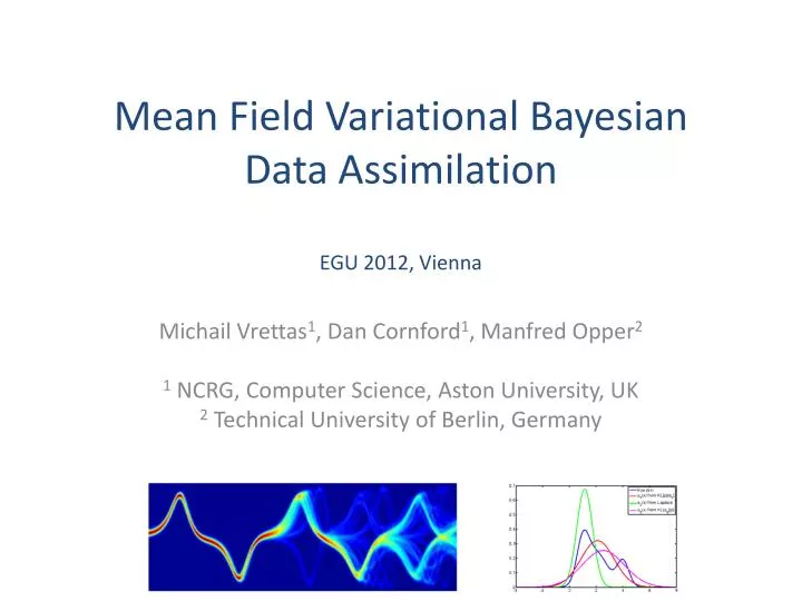
Mean Field Variational Bayesian Data Assimilation EGU 2012, Vienna. Michail Vrettas 1 , Dan Cornford 1 , Manfred Opper 2 1 NCRG, Computer Science, Aston University, UK 2 Technical University of Berlin, Germany. Why do data assimilation?.

E N D
Mean Field Variational Bayesian Data AssimilationEGU 2012, Vienna Michail Vrettas1, Dan Cornford1, Manfred Opper2 1 NCRG, Computer Science, Aston University, UK 2 Technical University of Berlin, Germany
Why do data assimilation? • Aim of data assimilation is to estimate the posterior distribution of the state of a dynamical model (X) given observations (Y) • may also be interested in parameter (θ) inference
Framing the problem • Need to consider: • model equations and model error: • observation and representativityerror: • Take a Bayesian approach: • This is an inference problem • exact solutions are hard; analytical impossible • approximations: MCMC, SMC, sequential (EnKF)
Our solution • Assume the model can be represented by a SDE (diffusion process): • We adopt a variational Bayesian approach • replace inference problem with an optimisation problem: find the best approximating distribution • best in sense of minimising the relative entropy (KL divergence) between true and approximating distribution • Question now is choice of approximating distributions
On the choice of approximations • We look for a solution in the family of non-stationary Gaussian processes • equivalent to time varying linear dynamical system • add a mean field assumption, i.e. posterior factorises • parameterise the posterior continuous time linear dynamical system using low order polynomials between observation times • This gives us an analytic expression for cost function (free energy) and gradients • no need for forwards / backwards integration
On algorithm complexity • Derivation of cost function equations challenging – but much can be automated • Memory complexity <full weak constraint 4D VAR • need to store parameterised means and variances • Time complexity > weak constraint 4D VAR • integral equations are complex, but can be solved analytically: no adjoint integration is needed • Long time windows are possible • provides a bound on marginal likelihood, thus approximate parameter inference is possible
Relation to other methods • This is a probabilistic method – targets the posterior, thus mean optimal • 4D VAR (except Eyink’s work) targets the mode • Works on full time window; not sequential like EnKF and PF approaches • no sampling error, but still have approximation error • Probably most suited for parameter estimation
Limitations • Mean field => no correlations! • note correlations in model and reality still there, approximation only estimates marginally • Variational => no guarantees on approximation error • empirically we see this is not a problem, comparing with very expensive HMC on low dimensional systems • Parameterisation => much be chosen • Gaussian assumption on approximation, not true posterior • quality of approximation depends on closeness to Gaussian • Implementation => model specific • need to re-derive equations if model changes, but automation possible
Conclusions • Mean field methods make variational Bayesian approaches to data assimilation possible for large models • main benefit is parameter inference with long time windows • next steps test for inference of observation errors Acknowledgement: This work was funded by the EPSRC (EP/C005848/1) and EC FP7 under the GeoViQua project (ENV.2010.4.1.2-2; 265178)