Download
1 / 59
610 likes | 866 Views
Asymptotic Analysis. Asymptotic Analysis. Suppose we have two algorithms, how can we tell which is better? We could implement both algorithms, run them both. Asymptotic Analysis. Suppose a company has Algorithm A implemented, tested, and shipped

E N D
Asymptotic Analysis • Suppose we have two algorithms, how can we tell which is better? • We could implement both algorithms, run them both
Asymptotic Analysis • Suppose a company has Algorithm A implemented, tested, and shipped • An employee comes up with an improved version, Algorithm B • Implementing and testing Algorithm B may take a number of weeks (implementation, documentation, and testing)
Asymptotic Analysis • Without algorithm analysis, there will always be lingering questions: • Was the algorithm implemented correctly? • Are there any bugs? • How much faster?
Asymptotic Analysis • You may have heard that on your work-term reports, you should use quantitative analysis instead of qualitative analysis • The second refers to comparison of qualities, e.g., faster, less memory, etc. • Engineers must determine the actual costs involved with the algorithms they propose
Asymptotic Analysis • Suppose we had an algorithm which was, on average twice as slow • If the implementation of a new algorithm required two weeks of implementation, one if integration, one week of documentation, and one week of testing, this would total $10 000 in salaries • These are exceptionally conservative estimations
Asymptotic Analysis • With that same amount of money, you could purchase a computer which was twice as fast
Asymptotic Analysis • There are other algorithms which are significantly faster as the problem size increases • Given sorted lists of size 7, 15, 31, and 63 • a linear search requires 4, 8,16, and 32 inspections, respectively • a binary search requires 3, 4, 5, and 6 inspections, respectively
Asymptotic Analysis • In general, we will always analyze algorithms with respect to one or more variables • These variables may represent • the number of items (n) currently stored in an array or other data structure • the number of items expected to be stored in an array or other data structure • the dimensions of a matrix (n × n) or vector (n)
Asymptotic Analysis • For example, the time taken to find the largest object in an array of n random integers will take n operations int find_max( int * array, int n ) { int max = array[0]; for ( int i = 1; i < n; ++i ) { if ( array[i] > max ) { max = array[i]; } } return max; }
Asymptotic Analysis • One comment: • in this class, we will look at both simple C++ arrays and the standard template library (STL) structures • instead of using the primitive array, we could use the STL vector class • the vector class is closer to the C#/Java array
Asymptotic Analysis #include <vector> using namespace std; int find_max( vector<int> array ) { if ( array.size() == 0 ) { throw underflow(); } int max = array[0]; for ( int i = 1; i < array.size(); ++i ) { if ( array[i] > max ) { max = array[i]; } } return max; }
Asymptotic Analysis • Given data structures and algorithms: • we were able to determine this from the description of the algorithm • our goal will be to perform this mathematically
Asymptotic Analysis • Consider the two functions f(n) = n2 and g(n) = n2 – 3n + 2 • Around n = 0, they look very different
Asymptotic Analysis • If we look at a slightly larger range fromn = [0, 10], we begin to note that they are more similar:
Asymptotic Analysis • Extending the range to n = [0, 100], the similarity increases:
Asymptotic Analysis • And on the range n = [0, 1000], they are (relatively) indistinguishable:
Asymptotic Analysis • The are different absolutely, for example, f(1000) = 1 000 000 g(1000) = 997 002 however, the relative difference is very small and this difference goes to zero as n →∞
Asymptotic Analysis • To demonstrate with another example, f(n) = n6 and g(n) = n6 – 23n5+193n4 –729n3+1206n2 – 648n2 – 3n + 2 • Around n = 0, they are very different
Asymptotic Analysis • Even extending the range to n = [0, 10] does not appear to give much similarity
Asymptotic Analysis • However, as we extend the range, they appear to look a lot more similar:
Asymptotic Analysis • And finally, around n = 1000, the relative difference is less than 3%
Asymptotic Analysis • The justification for both pairs of polynomials being similar is that, in both cases, they each had the same leading term: • n2 in the first case, and • n6 in the second
Asymptotic Analysis • Suppose however, that the coefficients of the leading terms were different • In this case, both functions would exhibit the same rate of growth, however, one would always be proportionally larger
Asymptotic Analysis • Suppose we had two algorithms which sorted a list of size n and the number of machine instructions was given by f(n) = 35n2 + 230n + 432 g(n) = 42n2 + 130n + 372 • For small values of n, f(n) > g(n), however, for integral values of n > 14, g(n) > f(n)
Asymptotic Analysis • Thus, we can plot the number of machine instructions required to sort a list of size n • For small values of n, g(n) requires less work:
Asymptotic Analysis • With larger problems, the first algorithm, f(n), requires fewer instructions
Asymptotic Analysis • However, as we try to sort larger and larger lists, the difference in work is essentially proportional to the leading coefficients
Asymptotic Analysis • With n = 1000, g(n) is approximately equal to 42/35 g(n) = 1.2 g(n)
Asymptotic Analysis • Is this a serious difference between these two algorithms? • Because we can count the number instructions, we can also estimate how much time is required to run one of these algorithms on a computer
Asymptotic Analysis • Suppose we have a 1 GHz computer • Then the time required (in seconds) to sort a list of n objects is:
Asymptotic Analysis • With lists of size 10000, it still only takes 3.5 and 4.2 seconds, respectively:
Asymptotic Analysis • To sort a list with one million elements, it will take approximately 10 h to sort:
Asymptotic Analysis • With a problem of this size, the first algorithm takes just under 2 h less • Does this mean that we should not use the second algorithm? • Suppose we run the second algorithm on a 2 GHz computer
Asymptotic Analysis • By using a faster computer for the slower algorithm, the apparently poorer performing algorithm finishes sooner
Asymptotic Analysis • Of course, we could run both algorithms on the faster computer, however consider this scenario: • the 2nd (slower) algorithm is already implemented • development for the 1st (faster) algorithm would require 10 wk, including: implementation integration testing documenation
Asymptotic Analysis • Is it always the case that, given two polynomials of the same degree, it will always be possible to run the same algorithm on a faster machine • Justification? • if f(n) and g(n) are polynomials of the same degree then where
Asymptotic Analysis • Given any two functions f(n) and g(n), we will restrict ourselves to monotonically increasing functions • We will consider the limit of the ratio:
Asymptotic Analysis • If the two function f(n) and g(n) describe the run times of two algorithms, and that is, the limit is a constant, then we can always run the slower algorithm on a faster computer to get similar results
Asymptotic Analysis • To formally describe equivalent run times, we will say that f(n) = Q(g(n)) if • Note: this is not equality – it would have been better if it said f(n) ∈Q(g(n)) however, someone picked =
Asymptotic Analysis • We are also interested if one algorithm runs either asymptotically slower or faster than another • If this is true, we will say that f(n) = O(g(n))
Asymptotic Analysis • If the limit is zero, i.e., then we will say that f(n) = o(g(n)) t • This is the case if f(n) and g(n) are polynomials where f has a lower degree
Asymptotic Analysis • We have one final case:
Asymptotic Analysis • Usually, however, we are only interested if • one function is either as fast or faster than another function, or • one function is as slow as or slower than another function
Asymptotic Analysis • To summarize:
Asymptotic Analysis • That is: f(n) = O(g(n)) as being equivalent to f(n) = Q(g(n)) or f(n) = o(g(n)) and f(n) = W(g(n)) as begin equivalent to f(n) = Q(g(n)) or f(n) = w(g(n))
Asymptotic Analysis • Graphically, we can summarize these as follows: We say if
Asymptotic Analysis • Some other observations we can make are: f(n) = Q(g(n)) ⇔ g(n) = Q(f(n)) f(n) = O(g(n)) ⇔ g(n) = W(f(n)) f(n) = o(g(n)) ⇔ g(n) = w(f(n))
Asymptotic Analysis • By the properties of limits, we have that the relationship f(n) = Q(g(n)) is an equivalence relation: 1. f(n) = Q(g(n)) if and only if g(n) = Q(f(n)) 2. f(n) = Q(f(n)) 3. If f(n) = Q(g(n)) and g(n) = Q(h(n)), then f(n) = Q(h(n))
Asymptotic Analysis • Consequently, we can divide all functions into equivalence classes, where all functions within one class are big-Q of each other