Download
1 / 22
220 likes | 409 Views
Readings: K&F: 6.1, 6.2, 6.3, 14.1, 14.2, 14.3, 14.4, . Kalman Filters Gaussian MNs. Graphical Models – 10708 Carlos Guestrin Carnegie Mellon University December 1 st , 2008. Multivariate Gaussian. Mean vector:. Covariance matrix:. Conditioning a Gaussian. Joint Gaussian:

E N D
Readings: K&F: 6.1, 6.2, 6.3, 14.1, 14.2, 14.3, 14.4, Kalman FiltersGaussian MNs Graphical Models – 10708 Carlos Guestrin Carnegie Mellon University December 1st, 2008
Multivariate Gaussian Mean vector: Covariance matrix:
Conditioning a Gaussian • Joint Gaussian: • p(X,Y) ~ N(;) • Conditional linear Gaussian: • p(Y|X) ~ N(mY|X; s2Y|X)
Gaussian is a “Linear Model” • Conditional linear Gaussian: • p(Y|X) ~ N(0+X; s2)
Conditioning a Gaussian • Joint Gaussian: • p(X,Y) ~ N(;) • Conditional linear Gaussian: • p(Y|X) ~ N(mY|X; SYY|X)
Conditional Linear Gaussian (CLG) – general case • Conditional linear Gaussian: • p(Y|X) ~ N(0+BX; SYY|X)
Understanding a linear Gaussian – the 2d case • Variance increases over time (motion noise adds up) • Object doesn’t necessarily move in a straight line
Tracking with a Gaussian 1 • p(X0) ~ N(0,0) • p(Xi+1|Xi) ~ N( Xi + ; Xi+1|Xi)
Tracking with Gaussians 2 – Making observations • We have p(Xi) • Detector observes Oi=oi • Want to compute p(Xi|Oi=oi) • Use Bayes rule: • Require a CLG observation model • p(Oi|Xi) ~ N(W Xi + v; Oi|Xi)
Operations in Kalman filter X1 X2 X3 X4 X5 • Compute • Start with • At each time step t: • Condition on observation • Prediction (Multiply transition model) • Roll-up (marginalize previous time step) • I’ll describe one implementation of KF, there are others • Information filter O1 = O2 = O3 = O4 = O5 =
Exponential family representation of Gaussian: Canonical Form
Canonical form • Standard form and canonical forms are related: • Conditioning is easy in canonical form • Marginalization easy in standard form
Conditioning in canonical form • First multiply: • Then, condition on value B = y
Operations in Kalman filter X1 X2 X3 X4 X5 • Compute • Start with • At each time step t: • Condition on observation • Prediction (Multiply transition model) • Roll-up (marginalize previous time step) O1 = O2 = O3 = O4 = O5 =
Prediction & roll-up in canonical form • First multiply: • Then, marginalize Xt:
What if observations are not CLG? • Often observations are not CLG • CLG if Oi = Xi + o + • Consider a motion detector • Oi = 1 if person is likely to be in the region • Posterior is not Gaussian
Linearization: incorporating non-linear evidence • p(Oi|Xi) not CLG, but… • Find a Gaussian approximation of p(Xi,Oi)= p(Xi) p(Oi|Xi) • Instantiate evidence Oi=oi and obtain a Gaussian for p(Xi|Oi=oi) • Why do we hope this would be any good? • Locally, Gaussian may be OK
Linearization as integration • Gaussian approximation of p(Xi,Oi)= p(Xi) p(Oi|Xi) • Need to compute moments • E[Oi] • E[Oi2] • E[Oi Xi] • Note: Integral is product of a Gaussian with an arbitrary function
Linearization as numerical integration • Product of a Gaussian with arbitrary function • Effective numerical integration with Gaussian quadrature method • Approximate integral as weighted sum over integration points • Gaussian quadrature defines location of points and weights • Exact if arbitrary function is polynomial of bounded degree • Number of integration points exponential in number of dimensions d • Exact monomials requires exponentially fewer points • For 2d+1 points, this method is equivalent to effective Unscented Kalman filter • Generalizes to many more points
Operations in non-linear Kalman filter X1 X2 X3 X4 X5 • Compute • Start with • At each time step t: • Condition on observation (use numerical integration) • Prediction (Multiply transition model, use numerical integration) • Roll-up (marginalize previous time step) O1 = O2 = O3 = O4 = O5 =
What you need to know about Gaussians, Kalman Filters, Gaussian MNs • Kalman filter • Probably most used BN • Assumes Gaussian distributions • Equivalent to linear system • Simple matrix operations for computations • Non-linear Kalman filter • Usually, observation or motion model not CLG • Use numerical integration to find Gaussian approximation • Gaussian Markov Nets • Sparsity in precision matrix equivalent to graph structure • Continuous and discrete (hybrid) model • Much harder, but doable and interesting (see book)