Download
1 / 24
• 240 likes • 431 Views
Dynamic Pricing under Strategic Consumption. Chunyang Tong Sriram Dasu Information & Operations Management Marshall School of Business University of Southern California Los Angeles CA 90089. No. Yes. Price discriminating is optimal (case I). Single price is optimal (case II). No.

E N D
Dynamic Pricing under Strategic Consumption Chunyang Tong Sriram Dasu Information & Operations Management Marshall School of Business University of Southern California Los Angeles CA 90089
No Yes Price discriminating is optimal (case I) Single price is optimal (case II) No Literature (case III) X ( case IV) Yes A Framework Consumers Strategic The Seller Capacitated Strategic Consumers: Anticipate prices and buying strategies of other buyers
Are Buyer’s Strategic? • Empirical Evidence: “The price reduction occurrence can sometimes mean a more reliable source to come back to, time and time again.” (http://www.buyersale.com/sale_info.html) • Experimental Evidence: Posted price market buyers withhold demand (Ruffle, 2000)
Period 2 Period 1 Problem Setting • A Seller (risk-neutral monopolist) has K units of product to sell in finite horizon • A pool of N risk-neutral consumers with heterogeneous valuation. Commonly known is the cdf G(v), • Single-unit demand per consumer • Consumers have anticipation of future prices and maximize their expected surplus • Excess demand is resolved via proportional rationing (inefficient rationing) mechanism • Since initial capacity K is exogenously given, cost is treated as sunk
Pricing Schemes & Information Structures • Two pricing schemes: Upfront pricing and contingent pricing • Two information structures: Common posteriors and common priors • Common priors: buyer has a conditional probability distribution based on his own valuation and a common prior
Uncapacitated Seller, Strategic Consumers • Upfront Pricing Scheme ( P2, P1) • Since consumers face no risk of stock-out, they simply choose • min(P2, P1) • Single-pricing Optimal • Randomized Pricing ( P2, F(P1)) • Due to common knowledge of market information ( K,N,G(v)), • Single Pricing Optimal
Period 2 Period 1 Upfront Pricing (P2,P1), deterministic demand With limited supply single pricing may not be optimal: Example: K=2, N=10, with valuation ( 100,40,35,30,28,26,25,23,21,20) Optimal Single Price Scheme: P*=100, with revenue = 100 Two Price Scheme ( P2, P1)=(82, 20), with revenue = 82 + 20 = 102
Upfront Pricing Scheme, Deterministic demand Two-price scheme is optimal Price Price Price Pc P3 P3 Pc P2 P2 P1 P1 Pc time time time Lemma: The optimal pricing scheme consists of two prices ( P2, P1). The clearing price Pc is located in between.
Period 2 Period 1 Upfront Pricing Scheme, Stochastic demand (common posteriors) Consumers’ Symmetric Bayesian Nash Equilibrium Strategy: Threshold Policy: Only buyers with valuation v y* will buy in the second last period. Others will defer to the last period. y* solves the following equation: p2(y)(y – p2) = p1(y)(y- p1) where: pi(y) : probability of the buyer getting the object in period i.
Upfront Pricing Scheme, Stochastic demand (common posteriors) • A unique structure of equilibrium • Conjecture: Threshold is unique • Provide sufficient conditions for the threshold to be unique • Numerically verified that it is unique for U(0,1)
Computational result for uniform distribution For uniform distribution (0,1), N=5-50, K=1-(N-1), P2 is increasing Function of y.
Computational result for uniform distribution The more scarce the product is, the larger gap between prices
Impact on Profitability ( P1 is fixed at 0.3 )
Asymptotic Results • Prices are monotone non-increasing • Upfront pricing scheme leads to a valuation-skimming process. It is strategically equivalent to declining price auction when the number of price changes approaches infinity. • When number of buyers approaches infinity, a single price ( close enough to the upper bound of valuations) almost guarantees a near-optimal profit.
Contingent Pricing Scheme (common posteriors) • Buyers and sellers have common knowledge • Seller determines price based on sales in previous period
LHS y* RHS P1 P2 Contingent Pricing Scheme (common posteriors) The consumers’ equilibrium strategy is again a threshold policy Consumers in period 2 will buy immediately if and only if The curves of LHS and RHS have only one crossing point y*
Contingent Pricing, Common Posterior • Prices may increase • Relative value of Dynamic Pricing depends on level of scarcity • Best for “moderate” levels of scarcity • When N is very large in the limit a single price is adequate
Extensions of Common Posterior Case Threshold policy and approach for computing optimal prices extend to: • Multiple periods • New buyers entering each period • Valuations changing over time (provided expected valuations are convex functions of time)
Limitation of Common Posterior Model • Static pricing policy is near-optimal if: 1) the support of distribution is bounded; 2) Common posteriors; 3) Large number of buyers • To relax the assumption of common posteriors, we can assume just common priors on distribution of distributions
Common Priors • Distribution on distributions • G(i) is the pdf for Gi(v) (distribution of observed valuations) • Posterior distribution of each buyers depends on his/ her observed value • Assumption: Gi(v) Gj(v), if i > j, where i and j are the observed valuations of two buyers.
Example of Common Priors • Prior distribution: N(m, sp) • Buyer with observed valuation v, believes that true mean m’ = v + e, where e is N(0 ,se). • The posterior distributions are: N(m v, s) where • m v = v*(s2p/(s2e+s2p)) + m*(s2e/(s2e+s2p)) • s = s2es2p/(s2e+s2p) ( The more you value the product, the more you believe others value)
Common Priors • If , then a threshold policy is a symmetric Nash Equilibrium.
Work in Progress • Terminal consumption: uncertain valuation until • the final period • Capacity Control along with pricing • Seller can strategically reduce supply • Multiple unit purchase • Multi-firm competition • Experimental Studies