Download
1 / 20
200 likes | 427 Views
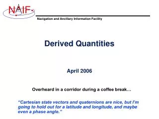
Derived Quantities. July 2013. What are Derived Quantities?. Derived quantities are produced using data from kernels These are the primary reason that SPICE exists! Examples are: Lighting conditions Surface intercept (LAT/LON) General geometry Coordinate system conversions

E N D
Derived Quantities July 2013
What are Derived Quantities? • Derived quantities are produced using data from kernels • These are the primary reason that SPICE exists! • Examples are: • Lighting conditions • Surface intercept (LAT/LON) • General geometry • Coordinate system conversions • Matrix and vector operations • The SPICE Toolkit contains many routines that assist with the computations of derived quantities. • Some are fairly low level, some are quite high level. • More are being added as time permits. Derived Quantities
A Quick Tour • Vector/Matrix Routines • Vector and vector derivative arithmetic • Matrix arithmetic • Geometric “Objects” • Planes • Ellipses • Ellipsoids • Rays • Coordinate Systems • Spherical: latitude/longitude, co-latitude/longitude, right ascension/declination; Geodetic, Cylindrical, Rectangular, Planetographic • Others (the most interesting ones!) • Lighting angles, sub-points, intercept points, season, geometric event finder The lists on the following pages are just a subset of what’s available in the Toolkit. Derived Quantities
Function <v,w> v x w v/|v| v x w / | v x w| v + w v - w av [+ bw [+ cu]] angle between v and w |v| v v | w VPROJ, VPERP v|| v TWOVEC, FRAME w Vectors • Routine • VDOT, DVDOT • VCROSS, DVCRSS • VHAT, DVHAT • UCROSS, DUCRSS • VADD, VADDG • VSUB, VSUBG • VSCL, [VLCOM, [VLCOM3]] • VSEP • VNORM Derived Quantities
Routine MXV MXM MTXV MTXM MXMT VTMV XPOSE INVERSE, INVSTM Matrices Selected Matrix-Vector Linear Algebra Routines • Function • M x v • M x M • Mt x v • Mt x M • M x Mt • vt x M x v • Mt • M-1 M = Matrix V = Vector X = Multiplication T = Transpose Derived Quantities
Function Routines Transform between Transform between Transform between Transform between 3x3 rotation matrix 3x3 rotation matrix 3x3 rotation matrix ax ay az 0 bx by bz cx cy cz EUL2M, M2EUL Q2M, M2Q xyz ax ay az xyz bx by bz xyz cx cy cz ax ay az ax ay az ax ay az bx by bz bx by bz bx by bz RAXISA, AXISAR ROTATE, ROTMAT cx cy cz cx cy cz cx cy cz Matrix Conversions Euler angles EUL2XF, XF2EUL RAV2XF, XF2RAV Euler angles and Euler angle rates or rotation matrix and angular velocity vector 6x6 state transformation matrix Rotation axis and angle (Q0,Q1,Q2,Q3) SPICE Style Quaternion Derived Quantities
Ellipsoids nearest point surface ray intercept surface normal limb slice with a plane altitude of ray w.r.t. to ellipsoid Planes intersect ray and plane Ellipses project onto a plane find semi-axes of an ellipse NEARPT, SUBPNT, DNEARP SURFPT, SINCPT SURFNM EDLIMB INELPL NPEDLN INRYPL PJELPL SAELGV Geometry Function Routine Derived Quantities
Coordinate Transformation Latitudinal to/from Rectangular Planetographic to/from Rectangular R.A. Dec to/from Rectangular Geodetic to/from Rectangular Cylindrical to/from Rectangular Spherical to/from Rectangular Routine LATREC RECLAT PGRREC RECPGR RADREC RECRAD GEOREC RECGEO CYLREC RECCYL SPHREC RECSPH Position Coordinate Transformations Derived Quantities
Coordinate Transformation Latitudinal to/from Rectangular Planetographic to/from Rectangular R.A. Dec to/from Rectangular Geodetic to/from Rectangular Cylindrical to/from Rectangular Spherical to/from Rectangular Jacobian (Derivative) Matrix Routine DRDLAT DLATDR DRDPGR DPGRDR DRDLAT* DLATDR* DRDGEO DGEODR DRDCYL DCYLDR DRDSPH DSPHDR * Jacobian matrices for the R.A and Dec to/from rectangular mappings are identical to those for the latitudinal to/from rectangular mappings Velocity Coordinate Transformations - 1 Derived Quantities
Velocity Coordinate Transformations - 2 • Example: transform velocities from rectangular to spherical coordinates using the SPICE Jacobian matrix routines. The SPICE calls that implement this computation are: CALL SPKEZR ( TARG, ET, REF, CORR, OBS, STATE, LT ) CALL DSPHDR ( STATE(1), STATE(2), STATE(3), JACOBI ) CALL MXV ( JACOBI, STATE(4), SPHVEL ) • After these calls, the vector SPHVEL contains the velocity in spherical coordinates: specifically, the derivatives ( d (r) / dt, d (colatitude) / dt, d (longitude) /dt ) • Caution: coordinate transformations often have singularities, so derivatives may not exist everywhere. • Exceptions are described in the headers of the SPICE Jacobian matrix routines. • SPICE Jacobian matrix routines signal errors if asked to perform an invalid computation. Derived Quantities
Other Derived Geometric Quantities • Illumination angles (phase, incidence, emission) • ILUMIN* • Subsolar point • SUBSLR* • Subobserver point • SUBPNT* • Surface intercept point • SINCPT* • Longitude of the sun (Ls), an indicator of season • LSPCN * These routines supercede the now deprecated routines ILLUM, SUBSOL, SUBPT and SRFXPT Derived Quantities
Most SPICE routines are used to determine a quantity at a specified time. The SPICE Geometry Finder (GF) subsystem takes the opposite approach: find times, or time spans, when a specified geometric condition or event occurs. This is such a large topic that a separate tutorial (“geometry_finder”) has been written for it. Geometric Events Finder Derived Quantities 12
Examples • On the next several pages we present examples of using some of the “derived quantity” APIs. Derived Quantities
Computing Illumination Angles • Given the direction of an instrument boresight in a bodyfixed frame, return the illumination angles (incidence, phase, emission) at the surface intercept on a tri-axial ellipsoid incidence phase emission instrument boresight direction target-observer vector Derived Quantities
Computing Illumination Angles • CALL GETFOV to obtain boresight direction vector • CALL SINCPT to find intersection of boresight direction vector with surface • CALL ILUMIN to determine illumination angles incidence phase emission instrument boresight direction target-observer vector Derived Quantities
Computing Ring Plane Intercepts • Determine the intersection of the apparent line of sight vector between Earth and Cassini with Saturn’s ring plane and determine the distance of this point from the center of Saturn. Derived Quantities
Computing Ring Plane Intercepts-2 This computation is for the reception case; radiation is received at the earth at a given epoch “ET”. • CALL SPKEZR to get light time corrected position of spacecraft as seen from earth at time ET in J2000 reference frame SCVEC. • CALL SPKEZR to get light time corrected position of center of Saturn at time ET as seen from earth in J2000 frame SATCTR. • CALL PXFORM to get rotation from Saturn body-fixed coordinates to J2000 at light time corrected epoch. The third column of this matrix gives the pole direction of Saturn in the J2000 frame SATPOL. • CALL NVP2PL and use SATCTR and SATPOL to construct the ring plane RPLANE. • CALL INRYPL to intersect the earth-spacecraft vector SCVEC with the Saturn ring plane RPLANE to produce the intercept point X. • CALL VSUB to get the position of the intercept with respect to Saturn XSAT (subtract SATCTR from X) and use VNORM to get the distance of XSAT from the center of Saturn. This simplified computation ignores the difference between the light time from Saturn to the earth and the light time from the ring intercept point to the earth. The position and orientation of Saturn can be re-computed using the light time from earth to the intercept; the intercept can be re-computed until convergence is attained. Derived Quantities 17
Computing Ring Plane Intercepts-3 • Create a dynamic frame with one axis pointing from earth to the light time corrected position of the Cassini orbiter. Use the CN correction for this position vector. (This gives us a frame in which the direction vector of interest is constant.) • Temporarily change the radii of Saturn to make the polar axis length 1 cm and the equatorial radii 1.e6 km. This can be done either by editing the PCK or by calling BODVCD to fetch the original radii, then calling PDPOOL to set the kernel pool variable containing the radii to the new values. This flat ellipsoid will be used to represent the ring plane. • Use SINCPT to find the intercept of the earth-Cassini ray with the flat ellipsoid. Use the CN correction. SINCPT returns both the intercept in the IAU_SATURN frame and the earth-intercept vector. Use VNORM to get the distance of the intercept from Saturn’s center. • Restore the original radii of Saturn. If PDPOOL was used to update the radii in the kernel pool, use PDPOOL again to restore the radii fetched by BODVCD. An alternate approach Derived Quantities 18
Direction to the observer Spacecraft motion A body such as a satellite Computing Occultation Events • Determine when the spacecraft will be occulted by an object (such as a natural satellite) as seen from an observer (such as earth). Derived Quantities
Direction to the observer Spacecraft motion A body such as a satellite Find Occultation Ingress/Egress • Select a start epoch, stop epoch and step size. • Start and stop epochs can bracket multiple occultation events • Step size should be smaller than the shortest occultation duration of interest, and shorter than the minimum interval between occultation events that are to be distinguished, but large enough to solve problem with reasonable speed. • Insert search interval into a SPICE window. This is the “confinement window.” • CALL GFOCLT to find occultations, if any. The time intervals, within the confinement window, over which occultations occur will be returned in a SPICE window. • GFOCLT can treat targets as ellipsoids or points (but at least one must be an ellipsoid). • GFOCLT can search for different occultation or transit geometries: full, partial, annular, or “any.” Derived Quantities