Long-Run Macroeconomic Equilibrium

1. Long-Run MacroeconomicEquilibrium And Government Policy

2. Economy is always at a point (PL & real GDP) on the SRAS curve. If that point is not also on the LRAS curve, the SRAS curve will shift until it is. Let’s consider three scenarios… SRAS to LRAS

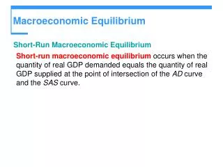
3. Long-Run Macro Equilibrium (#1) • Economy on both SRAS and LRAS curves • YE = YP

4. Inflationary Gap (#2) • Aggregate output above potential output • Results from positive AD shift Self-Correcting in the Long Run… • Low unemployment will lead to nominal wages rising, along with other “sticky” costs • Producers decrease output, bringing the economy back into equilibrium (at a higher price level)

5. Recessionary Gap (#3) • Aggregate output below potential output • Results from negative AD or negative SRAS shift Self-Correcting in the Long Run… • High unemployment will cause nominal wages to fall, along with other “sticky” costs • Producers increase output, bringing the economy back into equilibrium (at a lower price level)

6. Analysis of Gaps • Output gap – The difference between actual aggregate output and potential output Output gap = Actual aggregate output – Potential output X 100 Potential output

7. The Purpose of Macroeconomic Policy • Most economists believe that it takes the economy a decade or longer to self-correct • Economists like Keynes believe in active stabilization, use of government policy to reduce the severity and length of recessions or to rein in excessive expansions

8. Response to Demand Shocks • Fall in demand is easiest to correct through policy • Unfortunately, policy measures to increase AD can increase deficits & may hinder long-run growth • Government tries to offset positive shocks too, as inflationary gaps have significant costs in the long-run

9. Response to Supply Shocks • No easy remedy for these, as they result from changes in production costs • A negative supply shock leads to rising prices and decreasing output (& employment) • Policy to fix one of these problems makes the other worse

10. Governmental Circular Flow • Inflows – Taxes and borrowing • Outflows – Government purchases and transfers

11. GDP = C + I + G + X - IM • Government directly controls G, but also indirectly influences C and I through fiscal policy • C is based on disposable income, which is directly related to transfers and taxes • I is influenced by business regulation

12. Expansionary Fiscal Policy • To address a recessionary gap, the government attempts to increase AD: • Increase government purchases AND/OR • Cut taxes AND/OR • Increase transfers

13. Contractionary Fiscal Policy • To address an inflationary gap, the government attempts to decrease AD: • Reduce government purchases AND/OR • Raise taxes AND/OR • Reduce transfers

14. Lags in Fiscal Policy • Many economists argue against extremely active stabilization policies • One caution for fiscal policy is time lag • Government must acknowledge gap • Government has to develop a plan • Plan implementation

15. Multiplier Effect of Increasing Government Purchases • Government spending is an autonomous increase in aggregate spending • Money is spent again and again, so it is subject to the multiplier • Also the same multiplier for reduction

16. Multiplier Effect of Changes in Government Transfers & Taxes • Smaller effect than government purchases • Instead, change in GDP results from household spending – so its initial infusion is subject to the multiplier

17. Taxes and the Multiplier • Taxes capture part of the increase in real GDP • As a result of tax structure, government revenue increases when real GDP does

18. Types of Government Stabilizers • The overall result of tax policies is to reduce the multiplier, creating greater stability – so these are known as automatic stabilizers • Some government transfers are also automatic stabilizers, but active policies are discretionary fiscal policies