Download
1 / 42
420 likes | 529 Views
Chapter 24 Sorting Supplement. 7 2 9 4 2 4 7 9. 7 2 2 7. 9 4 4 9. 7 7. 2 2. 9 9. 4 4. Merge Sort. Divide-and-Conquer. Divide-and conquer is a general algorithm design paradigm

E N D
7 2 9 4 2 4 7 9 7 2 2 7 9 4 4 9 7 7 2 2 9 9 4 4 Merge Sort
Divide-and-Conquer • Divide-and conquer is a general algorithm design paradigm • Divide: If the input size is smaller than a certain threshold, solve the problem directly using a straightforward method and return the solution obtained, otherwise divide the input into two or more disjoint subsets • Recur: Recursively solve the sub-problems associated with the subsets • Conquer: Take the solution to the sub-problems and merge then into a solution to the original problem
Using Divide-and-Conquer for Sorting • A merge-sort on an input sequence S with n elements using a comparator consists of three steps based on the divide-and-conquer paradigm: • Divide: partition S into two sequences S1and S2 of about n/2 elements each • S1 contains the first elements and S2 contains the remaining elements • Recur: recursively sort S1and S2 • Conquer: merge S1and S2 into a sorted sequence
Merge-Sort Algorithm AlgorithmmergeSort(S, C) Input sequence S with n elements, comparator C Output sequence S sorted • according to C ifS.size() > 1 (S1, S2) partition(S, n/2) mergeSort(S1, C) mergeSort(S2, C) S merge(S1, S2)
7 2 9 4 2 4 7 9 3 8 6 1 1 3 8 6 7 2 2 7 9 4 4 9 3 8 3 8 6 1 1 6 7 7 2 2 9 9 4 4 3 3 8 8 6 6 1 1 Execution Example (1) • Partition 7 2 9 4 3 8 6 11 2 3 4 6 7 8 9
7 2 2 7 9 4 4 9 3 8 3 8 6 1 1 6 7 7 2 2 9 9 4 4 3 3 8 8 6 6 1 1 Execution Example (2) • Recursive call, partition 7 2 9 4 3 8 6 11 2 3 4 6 7 8 9 7 2 9 4 2 4 7 9 3 8 6 1 1 3 8 6
7 7 2 2 9 9 4 4 3 3 8 8 6 6 1 1 Execution Example (3) • Recursive call, partition 7 2 9 4 3 8 6 11 2 3 4 6 7 8 9 7 2 9 4 2 4 7 9 3 8 6 1 1 3 8 6 7 2 2 7 9 4 4 9 3 8 3 8 6 1 1 6
7 2 2 7 9 4 4 9 3 8 3 8 6 1 1 6 Execution Example (4) • Recursive call, base case 7 2 9 4 3 8 6 11 2 3 4 6 7 8 9 7 2 9 4 2 4 7 9 3 8 6 1 1 3 8 6 77 2 2 9 9 4 4 3 3 8 8 6 6 1 1
Execution Example (5) • Recursive call, base case 7 2 9 4 3 8 6 11 2 3 4 6 7 8 9 7 2 9 4 2 4 7 9 3 8 6 1 1 3 8 6 7 2 2 7 9 4 4 9 3 8 3 8 6 1 1 6 77 22 9 9 4 4 3 3 8 8 6 6 1 1
Execution Example (6) • Merge 7 2 9 4 3 8 6 11 2 3 4 6 7 8 9 7 2 9 4 2 4 7 9 3 8 6 1 1 3 8 6 7 22 7 9 4 4 9 3 8 3 8 6 1 1 6 77 22 9 9 4 4 3 3 8 8 6 6 1 1
Execution Example (7) • Recursive call, …, base case, merge 7 2 9 4 3 8 6 11 2 3 4 6 7 8 9 7 2 9 4 2 4 7 9 3 8 6 1 1 3 8 6 7 22 7 9 4 4 9 3 8 3 8 6 1 1 6 77 22 9 9 4 4 3 3 8 8 6 6 1 1
Execution Example (8) • Merge 7 2 9 4 3 8 6 11 2 3 4 6 7 8 9 7 2 9 42 4 7 9 3 8 6 1 1 3 8 6 7 22 7 9 4 4 9 3 8 3 8 6 1 1 6 77 22 9 9 4 4 3 3 8 8 6 6 1 1
Execution Example (9) • Recursive call, …, merge, merge 7 2 9 4 3 8 6 11 2 3 4 6 7 8 9 7 2 9 42 4 7 9 3 8 6 1 1 3 6 8 7 22 7 9 4 4 9 3 8 3 8 6 1 1 6 77 22 9 9 4 4 33 88 66 11
Execution Example (10) • Merge 7 2 9 4 3 8 6 11 2 3 4 6 7 8 9 7 2 9 42 4 7 9 3 8 6 1 1 3 6 8 7 22 7 9 4 4 9 3 8 3 8 6 1 1 6 77 22 9 9 4 4 33 88 66 11
Analysis of Merge-Sort • The height h of the merge-sort tree is O(log n) • at each recursive call we divide in half the sequence • The overall amount or work done at the nodes of depth i is O(n) • One partitions and merges 2i sequences of size n/2i • One makes 2i+1 recursive calls • The total running time of merge-sort is O(n log n)
7 4 9 6 2 2 4 6 7 9 4 2 2 4 7 9 7 9 2 2 9 9 Quick-Sort
Quick-Sort • Quick-sort is based on the divide-and-conquer paradigm where most of the work is done before the recursive calls • Divide: pick a random element x (called pivot) and partition S into (common practice is to the last element of S) • L storeselements less than x • E storeselements equal x • G storeselements greater than x • Recur: Recursively sort L and G • Conquer: Put back the elements into S by concatenating the elements of L, followed by elements of E,then followed by the elements of G
Quick-Sort x x L G E x
Quick-Sort Tree • An execution of quick-sort is depicted by a binary tree • Each node represents a recursive call of quick-sort and stores • Unsorted sequence before the execution and its pivot • Sorted sequence at the end of the execution • The root is the initial call 7 4 9 6 2 2 4 6 7 9 4 2 2 4 7 9 7 9 2 2 9 9
Execution Example (1) • Pivot selection 7 2 9 4 3 7 6 11 2 3 4 6 7 8 9 7 2 9 4 2 4 7 9 3 8 6 1 1 3 8 6 9 4 4 9 3 3 8 8 2 2 9 9 4 4
Execution Example (2) • Partition, recursive call, pivot selection 7 2 9 4 3 7 6 11 2 3 4 6 7 8 9 2 4 3 1 2 4 7 9 3 8 6 1 1 3 8 6 9 4 4 9 3 3 8 8 2 2 9 9 4 4
Execution Example (3) • Partition, recursive call, base case 7 2 9 4 3 7 6 11 2 3 4 6 7 8 9 2 4 3 1 2 4 7 3 8 6 1 1 3 8 6 11 9 4 4 9 3 3 8 8 9 9 4 4
Execution Example (4) • Recursive call, …, base case, join 7 2 9 4 3 7 6 11 2 3 4 6 7 8 9 2 4 3 1 1 2 3 4 3 8 6 1 1 3 8 6 11 4 334 3 3 8 8 9 9 44
Execution Example (5) • Recursive call, pivot selection 7 2 9 4 3 7 6 11 2 3 4 6 7 8 9 2 4 3 1 1 2 3 4 7 9 7 1 1 3 8 6 11 4 334 8 8 9 9 9 9 44
Execution Example (6) • Partition, …, recursive call, base case 7 2 9 4 3 7 6 11 2 3 4 6 7 8 9 2 4 3 1 1 2 3 4 7 9 7 1 1 3 8 6 11 4 334 8 8 99 9 9 44
Execution Example (7) • Join, join 7 2 9 4 3 7 6 1 1 2 3 4 67 7 9 2 4 3 1 1 2 3 4 7 9 7 1779 11 4 334 8 8 99 9 9 44
Bucket-Sort and Radix-Sort 1, c 3, a 3, b 7, d 7, g 7, e 0 1 2 3 4 5 6 7 8 9 B
Bucket-Sort • Let be S be a sequence of n (key, element) entries with keys within the range [0, N - 1] • Bucket-sort uses the keys as indices into an a bucket array that has cells indexed from 0 to N – 1 • Not based on comparisons • Phase 1: Each entry with k is placed into the bucket B[k] which is a sequence of entries with key k • Phase 2: After inserting each entry of sequence S into a B[k], the entries are moved back into S in sorted order by enumerating the contents of the buckets, B[i] where i=0,..,N-1 in order
Bucket-Sort Properties • Key-type Property • The keys are used as indices into an array and cannot be arbitrary objects • Stable Sort Property • The relative order of any two items with the same key is preserved after the execution of the algorithm • For any two entries (ki,xi) and (kj,xj) of S such that ki=kj and(ki,xi) precedes (kj,xj) in S before sorting (that is i < j), (ki,xi) will precede (kj,xj) after sorting
7, d 1, c 3, a 7, g 3, b 7, e 1, c 3, a 3, b 7, d 7, g 7, e B 0 1 2 3 4 5 6 7 8 9 1, c 3, a 3, b 7, d 7, g 7, e Bucket-Sort Example • Key range [0, 9] Phase 1 Phase 2
Bucket-Sort Analysis: • Phase 1 takes O(n) time • Phase 2 takes O(n+ N) time • Bucket-sort takes O(n+ N) time • Where S is a sequence of n (key, element) entries with keys within the range [0, N - 1]
Lexicographic Order • Suppose one wants to sort entries with keys that are pairs (k,l) where k and l are integers in the range [0,N-1] • A lexicographic order on these keys: (k1,l1) < (k2,l2) if k1< k2 or k1= k2 and l1< l2
Lexicographic Order (Generalized) • A d-tuple is a sequence of d keys (k1, k2, …, kd), where key ki is said to be the i-th dimension of the tuple • Example: • The Cartesian coordinates of a point in space are a 3-tuple • The lexicographic order of two d-tuples is recursively defined as follows (x1, x2, …, xd) < (y1, y2, …, yd)x1 < y1 or x1 = y1 and(x2, …, xd) < (y2, …, yd) i.e., the tuples are compared by the first dimension, then by the second dimension, etc.
Overview of the Radix-Sort • Sort a sequence S with keys that are pairs (k,l) • Applies a stable bucket-sort twice • First using one component of the pairs as the ordering key • Second using the other component
Radix-Sort Example S=(3,3) (1,5) (2,5) (1, 2) (2, 3) (1,7) (3, 2) (2, 2) Using the first component S1=(1,5) (1,2) (1,7) (2, 5) (2, 3) (2,2) (3, 3) (3, 2) Then using the second component S1,2=(1,2) (2,2) (3,2) (2, 3) (3, 3) (1,5) (2, 5) (1, 7) Using the second component S2=(1,2) (3,2) (2,2) (3, 3) (2, 3) (1,5) (2, 5) (1, 7) Then using the first component S2,1=(1,2) (1,5) (1,7) (2, 2) (2, 3) (2,5) (3, 2) (3, 3) S2,1 is lexicographically ordered (using the second component then the first component)
Radix-Sort Summary • Radix-sort is a specialization of lexicographic-sort that uses bucket-sort as the stable sorting algorithm in each dimension • Radix-sort is applicable to d-tuples with keys (k1, k2, …, kd) in the range [0, N- 1] • Radix-sort runs in time O(d( n+ N))
Radix-Sort for Binary Numbers • Consider a sequence of nb-bit integers x=xb- 1 … x1x0 • We represent each element as a b-tuple of integers in the range [0, 1] and apply radix-sort with N= 2 • This application of the radix-sort algorithm runs in O(bn) time • For example, we can sort a sequence of 32-bit integers in linear time
1001 0001 1001 1001 0010 1101 0010 0010 0001 1110 0001 1101 0010 1001 1001 0010 1101 0001 1101 1101 1110 1110 1110 1110 0001 Sorting a Sequence of 4-bit integers input output
Merge-Sort Tree • An execution of merge-sort is depicted by a binary tree, T • Each node represents a recursive call of merge-sort algorithm • Each node v of T is processed by the call associated with v • The children of node v are associated with the recursive call that process the subsequences S1 and S2 • Unsorted sequence before the execution • Sorted sequence at the end of the execution • The external nodes are associated with the individual elements of S • The root is the initial call 7 2 9 4 2 4 7 9 7 2 2 7 9 4 4 9 7 7 2 2 9 9 4 4