Download
1 / 42
460 likes | 700 Views
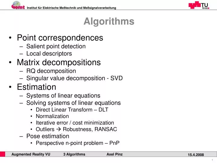
Algorithms. Point correspondences Salient point detection Local descriptors Matrix decompositions RQ decomposition Singular value decomposition - SVD Estimation Systems of linear equations Solving systems of linear equations Direct Linear Transform – DLT Normalization

E N D
Algorithms • Point correspondences • Salient point detection • Local descriptors • Matrix decompositions • RQ decomposition • Singular value decomposition - SVD • Estimation • Systems of linear equations • Solving systems of linear equations • Direct Linear Transform – DLT • Normalization • Iterative error / cost minimization • Outliers Robustness, RANSAC • Pose estimation • Perspective n-point problem – PnP
Point Correspondences - Example 1 Structure and motion from “natural” landmarks [Schweighofer] Stereo reconstruction of Harris corners
Point Correspondences - Example 2 elliptical support normalization “canonical view” correspondence [Mikolajczyk+Schmid]
Salient points (corners) based on 1st derivatives • Autocorrelation of 2D image signal [Moravec] • Approximation by sum of squared differences (SSD) • Window W • Differences between grayvalues in W and a window shifted by (Δx,Δy) • Four different shift directions fi(x,y): • A corner is detected, when fMoravec>th
Salient points (corners) based on 1st derivatives • Autocorrelation (second moment) matrix: • Avoids various shift directions • Approximate I(xw+Δx,yw+Δy) by Taylor expansion: • Rewrite f(x,y): “second moment matrix M”
Salient points (corners) based on 1st derivatives • Autocorrelation (second moment) matrix: • M can be used to derive a measure of “cornerness” • Independent of various displacements (Δx,Δy) • Corner: significant gradients in >1 directions rank M = 2 • Edge: significant gradient in 1 direction rank M = 1 • Homogeneous region rank M = 0 • Several variants of this corner detector: • KLT corners, Förstner corners
Salient points (corners) based on 1st derivatives • Harris corners • Most popular variant of a detector based on M • Local derivatives with “derivation scale” σD • Convolution with a Gaussian with “integration scale” σI • MHarris for each point x in the image • Cornerness cHarris does not require to compute eigenvalues • Corner detection: cHarris > tHarris
Salient points (corners) based on 1st derivatives • Harris corners
Salient points (corners) based on 2nd derivatives • Hessian determinant • Local maxima of det H [Beaudet] • Zero crossings of det H [Dreschler+Nagel] • Detectors are related to curvature • Invariant to rotation • Similar cornerness measure: local maxima of K [Kitchen+Rosenfeld]
Salient points (corners) based on 2nd derivatives • DoG / LoG [Marr+Hildreth] • Zero crossings • “Mexican hat”, “Sombrero” • Edge detector ! • Lowe’s DoG keypoints [Lowe] • Edge zero-crossing • Blob at corresponding scale: local extremum ! • Low contrast corner suppression: threshold • Assess curvature distinguish corners from edges • Keypoint detection:
Salient points (corners) without derivatives • Morphological corner detector [Laganière] • 4 structuring elements: +, ◊, x, □ • Assymetrical closing
Salient points (corners) without derivatives • SUSAN corners [Smith+Brady] • Sliding window • Faster than Harris
Salient points (corners) without derivatives • Kadir/Brady saliency [Kadir+Brady] • Histograms • Shannon entropy • Scale selection • Used in constellation model [Fergus et al.]
Salient points (corners) without derivatives • MSER – maximally stable extremal regions [Matas et al.] • Successive thresholds • Stability: regions “survive” over many thresholds
Affine covariant corner detectors • Locally planar patch affine distortion • Detect “characteristic scale” • see also [Lindeberg], scale-space • Recover affine deformation that fits local image data best elliptical support normalization “canonical view” correspondence [Mikolajczyk+Schmid]
Scaled Harris Corner Detector • “Harris Laplace” [Mikolajczyk+Schmid, Mikolajczyk et al.]
Scaled Hessian Detector • “Hessian Laplace” [Mikolajczyk+Schmid , Mikolajczyk et al.]
Harris Affine Detector • “Harris affine” [Mikolajczyk+Schmid , Mikolajczyk et al.]
Hessian Affine Detector • “Hessian affine” [Mikolajczyk+Schmid , Mikolajczyk et al.]
Qualitative comparison of detectors (1) Harris affine Harris Laplace Harris Hessian affine Hessian Laplace
Qualitative comparison of detectors (2) morphological Kadir/Brady MSER SUSAN
Descriptors (1) • Representation of salient regions • “descriptive” features feature vector • There are many possibilities ! • Categorization vs. specific OR, matching • Sufficient descriptive power • Not too much emphasis on specific individuals • Performance is often category-specific vs. AR ? feature vector extracted from patch Pn
Descriptors (2) • Grayvalues • Raw pixel values of a patch P • “local appearance-based description” • “local affine frame” LAF [Obdržálek+Matas] for MSER • General moments of order p+q: • Moment invariants: • Central moments μpq: invariant to translation
Descriptors (3) • Moment invariants: • Normalized central moments • Translation, rotation, scale invariant moments Φ1 ... Φ7 [Hu] • Geometric/photometric, color invariants [vanGool et al.] • Filters • “local jets” [Koenderink+VanDoorn] • Gabor banks, steerable filters, discrete cosine transform DCT
Descriptors (4) • SIFT descriptors [Lowe] • Scale invariant feature transform • Calculated for local patch P: 8x8 or 16x16 pixels • Subdivision into 4x4 sample regions • Weighted histogram of 8 gradient directions: 0º, 45º, … • SIFT vector dimension: 128 for a 16x16 patch [Lowe]
Algorithms • Point correspondences • Salient point detection • Local descriptors • Matrix decompositions • RQ decomposition • Singular value decomposition - SVD • Estimation • Systems of linear equations • Solving systems of linear equations • Direct Linear Transform – DLT • Normalization • Iterative error / cost minimization • Outliers Robustness, RANSAC • Pose estimation • Perspective n-point problem – PnP
RQ Decomposition (1) • Remember camera projection matrix P • P can be decomposed, e.g. finite projective camera
RQ Decomposition (2) • Unfortunately: R refers to “upper triangular”, Q to “rotation”… • “Givens rotations”: • How to decompose a given 3 x 3 matrix (say M) ? • MQx enforcingM32= 0, first column of M unchanged, last two columns replaced by linear combinations of themselves • MQxQy enforcing M31= 0, 2nd column unchanged (M32remains0) • MQxQyQz enforcing M21= 0, first two columns replaced by linear combinations of themselves, thus M31and M32remain0 MQxQyQz = R, M = RQxTQyTQzT , where R is upper triangular • How to enforce • e.g. M21= 0 ?
Singular Value Decomposition - SVD • Given a square matrix A (e.g. 3x3) • A can be decomposed into • where U and V are orthogonal matrices, and • D is a diagonal matrix with • non-negative entries, • entries in descending order. • “the column of V corresponding to the smallest singular value” • ↔ “the last column of V”
SVD (2) • SVD is also possible when A is non-square(e.g. m x n, m≥n) • A can again be decomposed into • where U is m x n with orthogonal columns (UTU=Inxn), • D is an n x n diagonal matrix with • non-negative entries, • entries in descending order, • V is an n x n orthogonal matrix.
SVD for Least-Squares Solutions • Overdetermined system of linear equations • Find least-squares ( algebraic error! ) solution • Algorithm: • Find the SVD • Set • Find • The solution is Even easier for Ax=0: “x is the last column of V”
Algorithms • Point correspondences • Salient point detection • Local descriptors • Matrix decompositions • RQ decomposition • Singular value decomposition - SVD • Estimation • Systems of linear equations • Solving systems of linear equations • Direct Linear Transform – DLT • Normalization • Iterative error / cost minimization • Outliers Robustness, RANSAC • Pose estimation • Perspective n-point problem – PnP
Systems of Linear Equations (1) • Estimation of • A homography H: • The fundamental matrix: • The camera projection matrix: • By finding n point correspondences • between 2 images • between image and scene • And solving a system of linear equations • Typical form: (2n x 9) / (2n x 12) matrix representing correspondences 9 - vector representing H, F 12 - vector representing P
Systems of Linear Equations (2) • How to obtain ? • Homography H • 3 x 3matrix, 8 DoF, non-singular • at least 4 point correspondences are required • Fundamental matrix F • 3 x 3 matrix, 7 DoF, rank 2 • at least 7 point correspondences are required • Camera projection matrix P • 3 x 4 matrix, 11 DoF, decomposition into K, R, t • at least 5-1/2 (6) point correspondences are required why ?
Homography Estimation (1) Point correspondences Equation defining the computation of H Some notation: Simple rewriting:
Homography Estimation (2) Ai is a 3 x 9 matrix , h is a 9-vector • the system describes 3 equations • the equations are linear in the unknown h • elements of Ai are quadratic in the known point coordinates • only 2 equations are linearly independent • thus, the 3rd equation is usually omitted [Sutherland 63]: Ai is a 2 x 9 matrix , h is a 9-vector
Homography Estimation (3) 1 point correspondence defines 2 equations H has 9 entries, but is defined up to scale 8 degrees of freedom at least 4 point correspondences needed • General case: • overdetermined • n point correspondences • 2n equations, A is a 2n x 9 matrix 4 x 2 equations
Camera Projection Matrix Estimation homography H: projection matrix P very similar ! • n point correspondences 2n equations that are linear in elements of P • A is a 2n x 12 matrix, entries are quadratic in point coordinates • p is a 12-vector • P has only 11 degrees of freedom • a minimum of 11 equations is required 5-1/2 (6) point correspondences
Fundamental (Essential) Matrix Estimation (1) • solving is different from solving • each correspondence gives only one equation in the coefficients of F ! • for n point matches we again obtain a set of linear equations (linear in f1-f9)
Fundamental (Essential) Matrix Estimation (2) • F is a 3 x 3 matrix,has rank 2, |F| = 0 F has only 7 degrees of freedom • at least 7 point correspondences are required to estimate F • Back to the solution of systems of linear equations ! similar systems of equations, but: different constraints
SVD for Least-Squares Solutions • Overdetermined system of linear equations • Find least-squares ( algebraic error! ) solution • Algorithm: • Find the SVD • Set • Find • The solution is Even easier for Ax=0: “x is the last column of V” This is also called “direct linear transform” – DLT
Relevant Issues in Practice • Poor condition of A Normalization • Algebraic error vs. • geometric error, Iterative minimization • nonlinearities (lens dist.) • Outliers Robust algorithms • (RANSAC)