Pathfinders for the SKA: Nlog (N) vs. N 2 Imaging

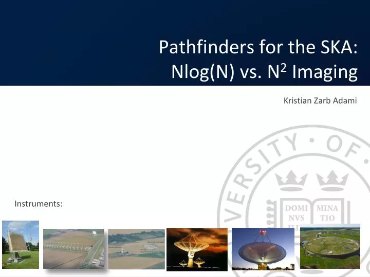
1. Pathfinders for the SKA:Nlog(N) vs. N2 Imaging KristianZarbAdami Instruments:

2. N log N Astronomy

3. In fact... • Japan designed the SKA in 1994 • 8x8 Images in 1994 with Waseda telescope • Extrapolating with Moore’s Law • (doubling every 18 months)  • 2016 is 1x106 antennas • Which is equivalent to SKA-phase-1

4. Remit of the talk • Science Justification for SKA1-Low • Science and Technical simulations towards implementation of the SKA • Physical Implementation on Medicinaas a flexible DSP test-bed and a comparison between spatial-FFT and N2 imaging • Industrial Engagement

5. SKA Phase-1 Specifications Memo 125

6. Sensitive (-ity) Issues.. [SKA Memo 100]

7. Roadmap to the SKA-lo SKA-1 N LOFAR Super Terp MWA-512 (400,50x2xNbeams) (8,50x2xNbeams) PAPER (32, 1024) (1,768) LOFAR UK (100,128) LWA MWA-32 (25,192) (78,100) GMRT (32, 64) (16,60) Medicina MITEOR (16,32) BW (25,16)

8. H1-Power Spectrum (z≈8) Theoretical 21-cm Power Spectrum @ 150 MHz Power Spectrum from a (100,256) instrument Foregrounds suppressed by frequency/angle differencing

9. NlogN vs. N2 SKA-Phase 1 Super-Terp 2011 SKA-Phase 2 LOFAR 2010

10. HI Power Spectra (SKA-Phase-II) Blue: HI > 108 Green: HI > 20’ Co-moving Volume = (500MPc/h)3 Linear Bias = 1.0 Linear bias = 0.8

11. SKA1 Low Layout 100km 200m

12. The numbers game (SKA1-low) • Bandwidth 70 – 450 MHz (Instantaneous B/W 380 MHz) • ADC Sampling at 1 GSa/s @ 8-bit • Antenna Spacing ~ 2.6m • Array Configuration: • 50 stations • 11,200 antennas per station (~10,000) • Output beams of 2-bit real; 2-bit imag

13. Numbers cont... • SKA-1 ~ 50 stations of 10,000 antennas each • Station diameter ≈ 200m • Station beam @ 70 MHz ≈ 1○, @ 450 MHz ≈ 0.2○ • Nbaselines= 5,000 (50^2/2 *4) • Input data rate to station 160 Tb/s (total data rate 8 Pb/s for the SKA-1 lo) • Output rate? • Assume 10 Tb/s off station = 100 x 100Gb/s fibres • Output beams 2+2 bits, ~100kHz channels (1.6Mbps per beam-channel) • 6.25 million beam-channels – by DFT need 0.1 Pop/s (6250 beams @ 1000 channels) • Equalise sky coverage so N(f) ~f2 – 100 beams in lowest (70 – 70.1 MHz) channel • 100 sq deg instantaneous coverage. • Correlator has to do 1,000 baselines for each 1 kHz beam-channel • (for a total ~ 10 Pop/s)

14. Station Architecture

15. Richard Armstrong – richard.armstrong@astro.ox.ac.uk Station Layout Copper Tile Processor Tile Processor Optical Fibre Optical Fibre Station Processor Tile Processor Tile Processor

16. Hierarchical Architecture Sub-Station Cross-correlation (calibration)? Hierarchical Beam Forming (tiles then station) Direct Station Beam Forming Antennas Tile Level Weights Station Weights Sub-Station Weights Electronic Calibration Field or Strong Source Calibration ~CAS-A Polarisation Calibration Tile level Station Level Weights Source & Polarisation Calibration Multiply and add by weights Multiply and add by weights Cross correlation of sub-arrays (for station calibration and ionospheric calibration)

17. Tile processor box RF in (coax) 16 x dual pol Fibre: Data out Clock and control in DC in Multi-chip module Reg

18. Tile Processor Tile Processor ADC Coarse freq splitting 1st Level Beamforming RFI Mitigation & 4-bit Quantisation Inputs: 16 dual-pol antennas ADC @ 1GSA/s @ 8-bit Coarse frequency splitting Into 4 channels Outputs: dual-polbeams @ 1GSA/s @ 4-bit re/4-bit imag Output is optical ADC ADC ADC Control and Calibration Interface

19. Space-Frequency Beamforming Time-delay beamforming is now an option… Dense mid-freq array: Antenna sep ~ 20cm Time step ~ 1ns ~ 30 cm Angle step > 45 deg Sparse low-freq array: Antenna sep ~2 m Time step ~ 1ns ~ 30 cm Angle step ~10 deg – less if interpolate Front end unit can combine space-freq beamforming in a single FIR-like structure Golden Rule: throw away redundant data before spending energy processing/transporting it

20. Station processor Electro-optical Electro-optical Electro-optical Electro-optical Electro-optical Heirarchical processor Heirarchical processor Heirarchical processor Heirarchical processor Heirarchical processor Optical-electro Optical-electro Optical-electro Optical-electro Optical-electro M&C M&C M&C M&C M&C Multi-chip module Multi-chip module Multi-chip module Multi-chip module Multi-chip module Clock & control

21. Station Processor 2nd Level Beamforming 2nd Level Channelisation Corner Turner Inputs: 64-dual pol 1st stage beams Outputs: selectable dual-pol beams @ 1GSA/s @ 2-bit re/2-bit imag Channelisation to 4096 channels With a 1024 channeliser Station Calibration and station correlator Output is optical and correlator ready Station Calibration and Correlator

22. Simulations

23. Multi-Level Beamforming • Split the problem to be hierarchical and parallel. • Station divided into tiles (can be logical). • Dump as much unwanted data as we can early on. Station beams Tile beam

24. Simple Beam Patterns 80 x 80 degrees: Tile beam at zenith. Station beam at (45, 87) degrees.

25. Visualisation of beams Elevation 85 - 90 degrees 1000 MHz65536 antennas, 256 tiles Station beams 0.20 degrees apart Tile beams 2 degrees apart 27 tile beams, 8005 station beams Run time: 2.18 seconds Station beams 0.05 degrees apart Tile beams 2 degrees apart 27 tile beams, 31707 station beamsRun time: 5.67 seconds

26. Dynamic Range Simulation Courtesy: S. Schediwy & Danny Price This is the reason a correlator is required for a beamformer

27. Array station sparsed x3 Auto-power beam Peak power 0 dB Cross-power beam 3deg rotation Peak power -20dB Cross-power beam 30 deg rotation Peak power -50dB

28. Examples of Implementation

29. Introduction Medicina Radio Telescopes 32m dish 564m 24 segments BEST-2 BEST-3Lo 640m 64 cylinders

30. Marco Bartolini, IRA - INAF BEST-2 specs

31. Medicina Radio Telescopes Richard B - ROACH 64- Channel ADC F - ROACH Griffin X - ROACH S - ROACH Jack Jack 1Gb-E PCI-X GPU Transient Alessio OeRC 10 Gb-e HOST - PC GPU Imaging & Calibration Dickie

32. Danny Price – Jack Hickish Medicina Backend: Spatial FFT

33. Medicina Fringes…

34. Medicina Fringes (Cas. A.)

35. Cas. A. Image

36. Industrial Engagement • It is NOT the intention of the SKA community to deliver 'finished' chip designs yet. • Aiming for detailed device specifications ready to start prototype manufacture when NRE money available • There are basic engineering processes that have to be done to enable meaningful sizing, cost & power estimation • IP identification and development – potential industrial involvement • Development of strategic technology partnerships • ADC design • IP macros for eg FFT, switch fabric • Embedded controllers • Non-packaged device mounting • Identification of key architectural features • Identify appropriate optimisation opportunities and trade-offs. • Development of accurate models for cost and power analysis at the wider system level. • Identify key interface 'Hot Spots' and apply effort accordingly

37. Industrial Engagement • Multi-Chip Module (One Chip to Rule them all!) • 4 x 4 antenna array (currently) – easily extended to 8x8 • Can also be used for Phased Array feeds for dishes • Current Chip RFI protection shows -57dB/m (in air) 10mW/ channel ?? 10mW/FFT 4mW/Beam RF IN Optical OUT Beam Combiner & Calibrator FIR-FFT Processor Optical I/O ADC 16-8 bit 1GS/s UWB RX 1024 channel splitter 16 element Beam combiner Optical Chip

38. Requirement Specifications