Download
1 / 16
160 likes | 176 Views
This study compares the measurements of solar irradiation in Romania with the numerical assessment methods. It explores the variability of solar power production and the implications for grid operators. It also discusses the historical perspective of solar radiation forecasting and the different numerical models used in forecasting. The study includes an evaluation of radiation models and their accuracy in predicting solar flux.

E N D
Comparison between measurements and numerical assessment of global solar irradiation in Romania DragosIsvoranu Viorel Badescu University Politehnica of Bucharest
Quality and performance of global solar • irradiance forecasting. Purpose Motivation • Variability of solar power production at different • spatial and temporal scales: • intermittent weather patterns • day/night cycles • humidity and aerosol load • cloud structure • Adapting the load schedule of grid operators • optimization of energy transport in low voltage grid • balancing energy; avoid outages and congestions • spot market sell ; penalties for wrong load schedules • maintenance planning • protection from extreme events
Historical perspective • contrary to wind forecasting, solar radiation forecasting is relatively new • 2008, Germany • 2011, Canada • significant reduction in RMSE with increasing the geographic area • under consideration in both cases • 2011, Spain, point forecast, RMSE between 10-50% depending on • cloudiness. Solar radiation forecasting • Forecasting horizon for PV: from 24 h up to 72 h. • In this range: numerical weather prediction based on equations of • fluid dynamics and thermodynamics to estimate the state of the • atmosphere at some time in the future. • NWP: Initialization: sample the state of the atmosphere at a given time • ( ground station, satellite, radar) • Time stepping: tens of minutes for global climate models to a few seconds • or minutes for regional models. • extrapolation methods (mainly for nowcasting) (global models) • statistical methods (up to 24 h horizon) (global models) • for regional models additional physics details
WRF presentation • NWP is stronly dependent on space scale • Meteorology scales: • global planetary (synoptic) • regional (mesoscale) (5- hundreds of km) • microscale (below 1 km) • Synoptic models: GFS, ECMWF, GME, UKMO • Mesoscale models: HRM, Hirlam, Lokal Model, WRF-(NMM, ARW), • Unified Model, MM5 • Selection of the numerical model: • popularity • cost • performance • accessibility to meteo and satellite data • European mesoscale codes: HRM, Hirlam, Lokal Model • semi-Lagrangian, semi-implicit formulation • North-American codes: WRF (ARW,NMM), MM5 • Eulerian formulation • Many pros and cons for each type of formulation • Though, a major failure for London Met Office for cloud propagation • from Eyjafjallajökul eruption in April 2010
WRF presentation • 2 dynamical nuclei: ARW (NCAR) and NMM (NCEP) • multigrid • multi-level • non-hidrostatic • LES turbulence model • space scales from tens of meters hundreds of km and even synoptic • one and bi-directional coupling with various physics modules • nested and moving grids • ARW : Arakawa-C type of grid • NMM : Arakawa-E type of grid • great flexibility and versatility by adding up new tailored modules • less numerical dissipation due to high order numerical algorithms • full parallelization • recent simulations showed similar accuracy compared to Unified Model • from UK Meteorological Office and GME from Deutsche Wetterdienst
Radiation model • radiation schemes: atmospheric heating and ground heat budget. • LW radiation: infrared radiation absorbed and emitted by gases and • surfaces. • Upward LW flux depends on the surface emissivity (land-use type, and ground (skin) temperature.) • SW radiation includes visible and surrounding wavelengths that make up • the solar spectrum. Hence, the only source is the Sun, but processes • include absorption, reflection, and scattering in the atmosphere and at • surfaces • Upward SW flux is the reflection due to surface albedo. • Within the atmosphere, radiation responds to model-predicted cloud and • water vapor distributions, as well as specified carbon dioxide, ozone. • All the radiation schemes in WRF currently are column (one-dimensional) • schemes(each column is treated independently), • Radiative fluxes are similar to those in infinite horizontally uniform planes • WRF options: • GFDL ; Lacis and Hansen (1974) • MM5 (Dudhia); Dudhia (1989) • Goddard Shortwave; Chou and Suarez (1994) • CAM Shortwave; NCAR Community Atmosphere Model (CAM 3.0)
Radiation model MM5 (Dudhia); • Simple downward integration of solar flux,. • Accounting for clear-air scattering, water vapor absorption (Lacis • and Hansen, 1974), and cloud albedo and absorption. • It uses look-up tables for clouds from Stephens (1978). • In WRF V3, the scheme has an option to account for terrain • slope and shadowing effects on the surface solar flux. cloud absorption and scattering absorption and scattering transmisivity • Evaluation of downward component of shortwave flux: • effects of solar zenith angle downward component and the path length; • clouds albedo and absorption; bilinearly interpolated from tabulated • functions. The total effect above height z percentage of Sd • clear air: scattering taken uniform and proportional to the atmosphere's • mass path length, again allowing for the zenith angle • water-vapour absorption as a function of water vapor path • (zenith angle)
ANM Timisoara station supplied with Kipp & Zonen CM6B radiometers. Results
WRF set-up • single-moment microphysics scheme following Hong et al. (2004) • the YSU planetary boundary layer scheme (Hong et al., 2006) • Kain–Fritsch cumulus scheme (Kain and Fritsch, 1993) • MM5 similarity based on Monin-Obukhov with Carslon-Boland • viscous sub-layer for surface layer (Paulson, 1970, Dyer and Hicks, • 1970 and Webb, 1970), • Unified Noah land-surface model, • RRTM scheme for long-wave radiation (Mlawer et al., 1997) • Dudhia scheme for shortwave radiation (Dudhia, 1989) • The synoptic meteorological data (GFS model) started on 06/13/2010- • 00:00:00 and expanded up to 06/20/2010-12:00:00 covering 180 hours • of forecast of the 0 cycle initialization. • Simulation domain centered on the geographical coordinates of radiometer • station and expands 1700 km in E-W direction and 850 km in N-S direction. • Grid spacing is 18.5 km. No nested grids. • The measured data consist of only 110 recordings covering the same forecast • horizon
red dots: simulation; black line: measurements; n: point-cloudiness ranging between 0 and 1.
Conclusions • GHI forecast fits well within experimental data for situations ranging • from clear sky to moderate cloudiness (n<= 0.7) • The statistics (MBE, RMSE) show 5%-10% larger values than • results of Lara-Fanego (2011) who used a different micro-physics • and grid step. Thank you for your patience