Download

1 / 27
300 likes | 365 Views
Explore the advancements in seismic inversion methods for recovering subsurface velocity structures using frequency domain formulations, full wave equations, and multi-scale approaches. This technical paper discusses the use of Maslov waveforms, ray sensitivity equations, regularization techniques, and closure constraints in the process. Gain insights into generating accurate velocity models through efficient waveform inversion strategies.

E N D
Aspects of seismic inversion Paul Childs *Schlumberger Cambridge Research With acknowledgements to: Colin Thomson*, ZhongMin Song †, Phil Kitchenside † Henk Keers* † Schlumberger WesternGeco, Gatwick HOP, Newton Institute, June 19th 2007
Survey configuration Marine seismic
Spectral interference notches from receiver-side free-surface ghost; O/U receivers allow for up/down separation, hence ghost removal; flatter, broader spectrum shows Earth structure better in seismic sections (=> better “attribute analysis”).
GPS Bird controller TRINAV Closing the loop TRIACQ StreamerSteering • Streamer control - with IRMA (Intrinsic Ranging by Modulated Acoustics) and Q-fin: GPS IRMA range data IRMA controller
velocity Seismic record time time Seismic “Image”
Complexity • Acoustic approximation is often made Ray methods: James Hobro, ChrisChapman, Henrik Bernth
Recover inhomogeneous subsurface velocity (density, impedance, …) field from surface measurements Born/Fréchet Kernel Green function from Full wave equation One-way wave equations Asymptotic ray theory Maslov Gaussian beam… (x,y) s r .x (Acoustic) Problem definition z s: source r: receiver x: scatterer/reflector
Fréchet kernels for multi-scale waveform inversion • Full wave equation inversion • Acoustic wave equation • Frequency domain • Helmholtz equation • Multigrid solver • Multiscale approach • Ray modeling • Turning waves • Maslov asymptotic approx. • Sensitivity, resolution & influence
Frequency domain formulation • Frequency domain adjoint formulation (Pratt): • Forward model: Forward propagation Back-propagation
f0 f1 f2 …. fn ….. Multi-scale approach* • Low frequency => large wavelength => large basin of convergence • Multiscale continuation • Solve for low frequency ~3 Hz • Increase frequencies incrementally • Use last [subsurface velocity] as initial guess for new frequency J *Sirgue, L and Pratt, R.G. (2004) “Efficient waveform inversion and imaging: A strategy for selecting temporal frequencies”, Geophysics 69(1), pp.231-248 *Pratt, R.G. et al (1998, 1999) *Ghattas et al. & Tromp et al
Exact velocity model Vp Vp Surface Depth Surface Depth Surface Depth Surface Surface Test model • Traveltime tomography starting model Surface Surface • Sensitivities
Inversion results f < 20 Hz Vp@ 1.5Hz Vp@ 5Hz Vp@ 16Hz Vp@ Truth
Inversion results Vp vs Depth Depth Offset 1/2 3/4 1/4
Optimization • Quasi-Newton, LBFGS • Solve for vp, ρ, source wavelet,… • Project constraints • L2, H2 + TV regularization • Gauss-Newton + line search • Constrained by modelling cost • Multiple right hand sides • Direct solver (SuperLU/MUMPS) • Multigrid solvers
Multigrid Preconditioner (Erlangga et al, 2006)* • H: Helmholtz • Indefinite • Not coercive • Non-local • C: Complex shifted Laplace, improved spectral properties • Preconditioner for H is C solved by Multigrid • *Y.A. Erlangga and C.W. Oosterlee and C. Vuik (2006). • “A Novel Multigrid Based Preconditioner For Heterogeneous Helmholtz Problems”, • SIAM J. Sci. Comput.,27, pp. 1471-1492, 2006
Multigrid Helmholtz solver - subsalt Multiple grids Vp Offset Depth Wavefield Sigsbee salt velocitymodel
X,p,T xr xs Plane wave synthesis receiver source
Results Initial velocity model • Low frequency starting model • caustics & pseudo-caustics Surface
Densified rays show stability even in such a complicated model; waveforms show back- scattering time time time CJT, 1999
Maslov* waveforms • Integral over plane waves • Sensitivity • Asymptotic theory *C.H.Chapman & R.Drummond, “Body-wave seismograms in inhomogeneous media using Maslov asymptotic theory”, Bull. Seism. Soc. America, vol 72, no. 6, pp.S277-S317, 1982.
Ray sensitivity equations (1) • Hamiltonian system • Dynamic ray tracing • Paraxial sensitivity
Ray tracing for gradients • Calculating the kernel • Solve ODEs • Propagator solves for • Sparse automatic differentiation evaluates
Basis functions Regularize over wavepaths Regularized gradient (5Hz) Fréchet derivatives
Gauss Newton Measures of resolution Offset • Resolution matrix • Posterior covariance • Lanczos solver • Hessian vector products only Diag(R) Depth Velocity model Vp Depth Offset
Closure • Frequency domain finite difference (FD) full waveform inversion • regularization • multi-scale optimization • Full wave equation FD(FE, SEM…) may be too detailed • reduced physics for forward models • Which approximations inform the inverse solution ? • Are Maslov waveforms effective for turning ray waveform inversion ? • Uncertainty estimates
End Comments ?