Download
1 / 22
220 likes | 239 Views
Learn about spatial resolution and quantization in digital image processing. Explore techniques, such as resampling and quantization methods like uniform quantization, dithering, and error diffusion. Understand how to alter resolution and enhance images using MATLAB commands.

E N D
Digital Image ProcessingLecture 3: Image Display & Enhancement Prof. Charlene Tsai
Spatial Resolution • The spatial resolution of an image is the physical size of a pixel in an image • Basically it is the smallest discernable detail in an image
Spatial Resolution (con’t) • The greater the spatial resolution, the more pixels are used to display the image. • How to alter the resolution using Matlab? • Imresize(x,n) • when n=1/2,
Spatial Resolution (con’t) • when n=2, • Commands that generate the images of slide2 • Imresize(imresize(x,1/2),2); • Imresize(imresize(x,1/4),4); • Imresize(imresize(x,1/8),8);
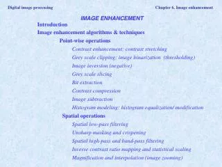
Quantization • Quantization refers to the number of greyscales used to represent the image. • A set of n quantization levels comprises the integers 0,1,2, …, n-1 • 0 and n-1 are usually black and white respectively, with intermediate levels rendered in various shades of gray. • Quantization levels are commonly referred to as gray levels • Sometimes the range of values spanned by the gray levels is called the dynamic range of an image.
Quantization (con’t) • n is usually an integral power of 2, n = 2b , where b is the number of bits used for quantization • Typically b=8 => 256 possible gray levels. • If b=1, then there are only two values: 0 and 1 (a binary image). • Uniform quantization: y=floor(double(x)/64); unit8(y*64); OR y=grayslice(x,4); Imshow(y,gray(4)); A mapping for uniform quantization
Quantization: Using “grayslice” image quantized to 8 greyscales image quantized to 4 greyscales image quantized to 2 greyscales
Method1: Dithering • Without dithering, visible contours can be detected between two levels. Our visual system is particularly sensitive to this. • By adding random noise to the original image, we break up the contouring. The quantization noise itself remains evenly distributed about the entire image. • The purpose: • The darker area will contain more black than white • The light area will contain more white than black • Method: Compare the image to a random matrix d
Dithering: Halftone • Using one standard matrix • Generate matrix d, which is as big as the image matrix, by repeating D. • The halftone image is >> r=repmat(D,128,128) >> x2=x>r; imshow(x2)
Dithering: General • Example: 4 levels • Step1: First quantize by dividing grey value x(i,j) by 85 (=255/3) • Suppose now that our replicated dither matrix d(i,j) is scaled so that its values are in the range 0 – 85 • The final quantization level p(i,j) is
Dithering: General x = imread('newborn.jpg'); % Dither to 4 greylevels D=[0 56;84 28]; r=repmat(D,128,128); x=double(x); q=floor(x/85); x4=q+(x-85*q>r); subplot(121); imshow(uint8(85*x4)); % Dither to 8 grey levels clear r x4 D=[0 24;36 12]; r=repmat(D,128,128); x=double(x); q=floor(x/37); x4=q+(x-37*q>r); subplot(122); imshow(uint8(37*x4)); 4 output greyscales 8 output greyscales
Method2: Error Diffusion • Quantization error: The difference between the original gray value and the quantized value. • If quantized to 0 and 255, Intensity value closer to the center (128) will have higher error.
(cont) • Goal: spread this error over neighboring pixels. • Method: sweeping from left->right, top->down, for each pixel • Perform quantization • Calculate the quantization error • Spread the error to the right and below neighbors
Error Diffusion Formulae • To spread the error, there are several formulae. • Weights must be normalized in actual implementation. Floyd-Steinberg
Error Diffusion Formulae • Matlab dither function implements the Floyd-Steinberg error diffusion Jarvis-Judice-Ninke Stucki
Summary • Quantization is necessary when the display device can handle fewer grayscales. • The simplest method (least pleasing) is uniform quantization. • The 2nd method is dithering by comparing the image to a random matrix. • The best method is error diffusion by spreading the error over neighboring pixels. • The chapter is from McAndraw. A copy will be placed online.
Image Enhancement • Two main categories: • Point operations: pixel’s gray value is changed without the knowledge of its surroundings. E.g. thresholding. • Neighborhood processing: The new gray value of a pixel is affected by its small neighborhood. E.g. smoothing. • We start with point operations.
Gray-level Slicing • Highlighting a specific range of gray levels. • Applications: • Enhancing specific features, s.t. masses of water in satellite images • Enhancing flows in X-ray images • Two basic approaches: • High value for all gray levels in the range of interest, and low value outside the range. • High value for all gray levels in the range of interest, but background unchanged.
Gray-level Slicing (con’t) Gonzales, section 3.2
Bit-plane Slicing • Highlighting the contribution made by specific bits. • Bit-plane 0 is the least significant, containing all the lowest order bits. • Bit-plane 7 is the most significant, containing all the highest order bits. • Higher-order bits contain visually significant data • Lower-order bits contain subtle details. • One application is image compression