Download
1 / 105
1.13k likes | 1.84k Views
Probability & Stochastic Processes for Communications: A Gentle Introduction. Shivkumar Kalyanaraman. Outline. Please see my experimental networking class for a longer video/audio primer on probability (not stochastic processes):

E N D
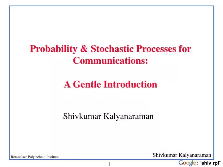
Probability & Stochastic Processes for Communications: A Gentle Introduction Shivkumar Kalyanaraman
Outline • Please see my experimental networking class for a longer video/audio primer on probability (not stochastic processes): • http://www.ecse.rpi.edu/Homepages/shivkuma/teaching/fall2006/index.html • Focus on Gaussian, Rayleigh/Ricean/Nakagami, Exponential, Chi-Squared distributions: • Q-function, erfc(), • Complex Gaussian r.v.s, • Random vectors: covariance matrix, gaussian vectors • …which we will encounter in wireless communications • Some key bounds are also covered: Union Bound, Jensen’s inequality etc • Elementary ideas in stochastic processes: • I.I.D, Auto-correlation function, Power Spectral Density (PSD) • Stationarity, Weak-Sense-Stationarity (w.s.s), Ergodicity • Gaussian processes & AWGN (“white”) • Random processes operated on by linear systems
Probability • Think of probability as modeling an experiment • Eg: tossing a coin! • The set of all possible outcomes is the sample space: S • Classic “Experiment”: • Tossing a die: S = {1,2,3,4,5,6} • Any subset A of S is an event: • A = {the outcome is even} = {2,4,6}
Probability of Events: Axioms •P is the Probability Mass function if it maps each event A, into a real number P(A), and: i.) ii.) P(S) = 1 iii.)If A and B are mutually exclusive events then, B A
S Probability of Events …In fact for any sequence of pair-wise-mutually-exclusive events, we have
Detour: Approximations/Bounds/Inequalities Why? A large part of information theory consists in finding bounds on certain performance measures
Approximations/Bounds: Union Bound • Applications: • Getting bounds on BER (bit-error rates), • In general, bounding the tails of prob. distributions • We will use this in the analysis of error probabilities with various coding schemes (see chap 3, Tse/Viswanath) A B P(A B) <= P(A) + P(B) P(A1 A2 … AN) <= i= 1..N P(Ai)
Approximations/Bounds: log(1+x) • log2(1+x) ≈ x for small x • Application: Shannon capacity w/ AWGN noise: • Bits-per-Hz = C/B = log2(1+ ) • If we can increase SNR () linearly when is small (i.e. very poor, eg: cell-edge)… • … we get a linear increase in capacity. • When is large, of course increase in gives only a diminishing return in terms of capacity: log (1+ )
Approximations/Bounds: Jensen’s Inequality Second derivative > 0
Schwartz Inequality & Matched Filter • Inner Product (aTx) <= Product of Norms (i.e. |a||x|) • Projection length <= Product of Individual Lengths • This is the Schwartz Inequality! • Equality happens when a and x are in the same direction (i.e. cos = 1, when = 0) • Application: “matched” filter • Received vector y = x + w (zero-mean AWGN) • Note: w is infinite dimensional • Project y to the subspace formed by the finite set of transmitted symbols x:y’ • y’ is said to be a “sufficient statistic” for detection, i.e. reject the noise dimensions outside the signal space. • This operation is called “matching” to the signal space (projecting) • Now, pick the x which is closest to y’ in distance (ML detection = nearest neighbor)
Conditional Probability • = (conditional) probability that the • outcome is in Agiven that we know the • outcome in B • Example: Toss one die. • Note that: What is the value of knowledge that B occurred ? How does it reduce uncertainty about A? How does it change P(A) ?
Independence • Events A and B are independent if P(AB) = P(A)P(B). • Also: and • Example: A card is selected at random from an ordinary deck of cards. • A=event that the card is an ace. • B=event that the card is a diamond.
Random Variable as a Measurement • Thus a random variable can be thought of as a measurement (yielding a real number) on an experiment • Maps “events” to “real numbers” • We can then talk about the pdf, define the mean/variance and other moments
Histogram: Plotting Frequencies Class Freq. Count 15 but < 25 3 25 but < 35 5 5 35 but < 45 2 4 Frequency Relative Frequency Percent 3 Bars Touch 2 1 0 0 15 25 35 45 55 Lower Boundary
Probability Distribution Function (pdf): continuous version of histogram a.k.a. frequency histogram, p.m.f (for discrete r.v.)
Continuous Probability Density Function • 1. Mathematical Formula • 2. Shows All Values, x, & Frequencies, f(x) • f(X) Is Not Probability • 3. Properties Frequency (Value, Frequency) f(x) f ( x ) dx 1 x a b All X (Area Under Curve) Value f ( x ) 0, a x b
Cumulative Distribution Function • The cumulative distribution function (CDF) for a random variable X is • Note that is non-decreasing in x, i.e. • Also and
Probability density functions (pdf) Emphasizes main body of distribution, frequencies, various modes (peaks), variability, skews
Cumulative Distribution Function (CDF) median Emphasizes skews, easy identification of median/quartiles, converting uniform rvs to other distribution rvs
Complementary CDFs (CCDF) Useful for focussing on “tails” of distributions: Line in a log-log plot => “heavy” tail
Numerical Data Properties Central Tendency (Location) Variation (Dispersion) Shape
Numerical DataProperties & Measures Numerical Data Properties Central Variation Shape Tendency Mean Range Skew Interquartile Range Median Mode Variance Standard Deviation
Expectation of a Random Variable: E[X] • The expectation (average) of a (discrete-valued) random variable X is
Continuous-valued Random Variables • Thus, for a continuous random variable X, we can define its probability density function (pdf) • Note that since is non-decreasing in x we have for all x.
Expectation of a Continuous Random Variable • The expectation (average) of a continuous random variable X is given by • Note that this is just the continuous equivalent of the discrete expectation
Other Measures: Median, Mode • Median= F-1 (0.5), where F = CDF • Aka 50% percentile element • I.e. Order the values and pick the middle element • Used when distribution is skewed • Considered a “robust” measure • Mode: Most frequent or highest probability value • Multiple modes are possible • Need not be the “central” element • Mode may not exist (eg: uniform distribution) • Used with categorical variables
Indices/Measures of Spread/Dispersion: Why Care? You can drown in a river of average depth 6 inches! Lesson: The measure of uncertainty or dispersion may matter more than the index of central tendency
Standard Deviation, Coeff. Of Variation, SIQR • Variance: second moment around the mean: • 2 = E[(X-)2] • Standard deviation = • Coefficient of Variation (C.o.V.)= / • SIQR= Semi-Inter-Quartile Range (used with median = 50th percentile) • (75th percentile – 25th percentile)/2
Covariance and Correlation: Measures of Dependence • Covariance: = • For i = j, covariance = variance! • Independence => covariance = 0 (not vice-versa!) • Correlation (coefficient) is a normalized (or scaleless) form of covariance: • Between –1 and +1. • Zero => no correlation (uncorrelated). • Note: uncorrelated DOES NOT mean independent!
Random Vectors & Sum of R.V.s • Random Vector = [X1, …, Xn], where Xi = r.v. • Covariance Matrix: • K is an nxn matrix… • Kij = Cov[Xi,Xj] • Kii = Cov[Xi,Xi] = Var[Xi] • Sum of independent R.v.s • Z = X + Y • PDF of Z is the convolution of PDFs of X and Y Can use transforms!
Captures all the moments, and is related to the IFT of pdf: Characteristic Functions & Transforms • Characteristic function: a special kind of expectation
Important (Discrete) Random Variable: Bernoulli • The simplest possible measurement on an experiment: • Success (X = 1) or failure(X = 0). • Usual notation: • E(X)=
Binomial Distribution n = 5 p = 0.1 Mean n = 5 p = 0.5 Standard Deviation
Binomial can be skewed or normal Depends upon p and n !
Binomials for different p, N =20 • As Npq >> 1, better approximated by normal distribution (esp) near the mean: • symmetric, sharp peak at mean, exponential-square (e-x^2) decay of tails (pmf concentrated near mean) 10% PER 30% PER Npq = 4.2 Npq = 1.8 50% PER Npq = 5
Important Random Variable:Poisson • A Poisson random variable X is defined by its PMF: (limit of binomial) Where > 0 is a constant • Exercise: Show that and E(X) = • Poisson random variables are good for countingfrequency of occurrence: like the number of customers that arrive to a bank in one hour, or the number of packets that arrive to a router in one second.
Important Continuous Random Variable: Exponential • Used to represent time, e.g. until the next arrival • Has PDF for some > 0 • Properties: • Need to use integration by Parts!
Gaussian/Normal Distribution References: Appendix A.1 (Tse/Viswanath) Appendix B (Goldsmith)
Gaussian/Normal • Normal Distribution: Completely characterized by mean () and variance (2) • Q-function: one-sided tail of normal pdf • erfc(): two-sided tail. • So:
Normal Distribution: Why? Uniform distribution looks nothing like bell shaped (gaussian)! Large spread ()! CENTRAL LIMIT TENDENCY! Sum of r.v.s from a uniform distribution after very few samples looks remarkably normal BONUS: it has decreasing !
Gaussian: Rapidly Dropping Tail Probability! Why? Doubly exponential PDF (e-z^2 term…) A.k.a: “Light tailed” (not heavy-tailed). No skew or tail => don’t have two worry about > 2nd order parameters (mean, variance) Fully specified with just mean and variance (2nd order)
Gaussian R.V. • Standard Gaussian : • Tail: Q(x) • tail decays exponentially! • Gaussian property preserved w/ linear transformations:
Standardize theNormal Distribution Normal Distribution Standardized Normal Distribution One table!
Obtaining the Probability Standardized Normal Probability Table (Portion) .02 .0478 0.1 .0478 Shaded area exaggerated Probabilities
ExampleP(X 8) Normal Distribution Standardized Normal Distribution .5000 .3821 .1179 Shaded area exaggerated
Q-function: Tail of Normal Distribution Q(z) = P(Z > z) = 1 – P[Z < z]