Download
1 / 27
270 likes | 411 Views
Adding 2 random variables that can be described by the normal model. AP Statistics B. Outline of lecture. Review of Ch 16, pp.376-78 (Adding or subtracting random variables that fit the normal curve)—last of Ch 16 Follow along in the text

E N D
Adding 2 random variables that can be described by the normal model AP Statistics B
Outline of lecture • Review of Ch 16, pp.376-78 (Adding or subtracting random variables that fit the normal curve)—last of Ch 16 • Follow along in the text • Remember that you can download this PowerPoint and a smaller, un-narrated one from the Garfield web site • Write down slide number if you don’t understand anything
First thing: make a picture, make a picture, make a picture! • Well, actually, a table, but a table IS a kind of picture, right?
Preliminaries: set-up and assumptions Setting up: NOTE: NOT time to get an entire box packed for sending; rather, we are only packing, not boxing! • P1=time for packing 1st stereo system • P2=time for packing NEXT stereo system • T=P1+P2 Assumptions: • Normal models for each RV • Both times independent of each other
Step one: calculate expected value (aka find the mean) • Remember that the expected value (EV) is a fancy word for finding the mean. • And with the mean, the EV sum of two random variables is the sum of their means:
Application to the packing and boxing problem • Mean (EV) of packing 1ST system is 9 min • Mean (EV) of packing 2nd system is also 9 min • Therefore:
Calculate standard deviation just like we have before • Nothing new, same old formula:
So what? • (You should always ask yourself “so what?” when somebody tells you to do something) • Well, we know that we had two RVs (random variables, not recreational vehicles; this is statistics, after all, not an auto show) that have a normal distribution. • So we now have a normal distribution and know the mean and standard deviation. • In statistical terms: N(18, 2.12) • Now we can evaluate this using what we learned in Ch. 6! A seriously big deal!
Q: What is the probability that packing 2 consecutive systems takes over 20 min? • This is the question we need to answer. • Remember the z-formula from Ch 6? • Write it down, and we’ll apply it on the next slide.
Setting up the problem • We already know the mean and standard deviation from our earlier calculations: 18 and 2.12, respectively. • The “y” value we are looking for is 20, so we set up the solution thusly:
Are we done yet? • Of course not. • Our goal is to find the probability that it will take MORE than 20 minutes to package 2 consecutive stereo systems. • The z-value of 0.94 simply means that the area to the LEFT of that point on the z-table (text, A79-A80) will be the probability that packaging will take LESS than 20 minutes.
Draw a picture! • The probability we get for z=0.94 is the dark blue area on the left. • However, we’re interested in the light blue area that’s ABOVE z=0.94
But first….. • Remember that our table only measures the cumulative probability to the LEFT of the value. • That’s all we have, so let’s find it, and then answer the question more directly.
How to use the table • It’s been a while, but get the X.x value on the inner column, and the 0.0x value across the top. The intersection is where the value lies, and looks like this:
Finding the probability to the left of 0.94 • Since 0.94>0, look on p. A-80 • Find 0.90 along the z-column on the far left • Read across the top row to 0.04 • The intersection of the 0.90 row and the 0.04 is the percentage of the normal curve to the LEFT of 0.94….. • ……which should be 0.8294
What are we looking for? • Not the blue area to the LEFT, but the clear area to the RIGHT of 0.94 • Calculate by subtracting the area to LEFT from 1: • 1.0000-0.8294=0.1706
Why the difference from the textbook? • Beats me. • But 0.1706 isn’t all THAT different from 0.1736…3 parts in a thousand.
Back to interpretation • We get a z-value of just over 17%. • That means, in everyday language, that there’s only a 17% chance (probability) that it will take more than 20 minutes to package 2 consecutive stereo systems. • NOTE: the AP exam expects you to write out things like this
What percentage of stereo systems take longer to back than to box? Next question(bottom of page 377)
Set-up on questions like this is crucial • The key is to realize that you don’t set it up as an inequality, exactly. • That is, the question is NOT P>B • Rather, the question is whether P-B>0. • We pick a different variable (D for “difference”) and define it as D=P-B
Why do we do it like this? • We now can ask a specific question, namely what’s the expected value of D? • In statistical terms, we have E(D)=E(P-B). • We can now calculate these values using what we’ve learned in Ch 16 and combining it with the normal model from Ch 6.
First the mean,then the standard deviation • E(D)=E(P-B)=E(P)-E(B) • E(P) we get from reading the mean for packing right off the table • We get E(B) the same way. • E(P)-E(B)=9 min – 3 min = 6 min
Calculating the standard deviation • I like to calculate the SD directly, but you can start with the variance, and then take the square root. • Var(D)=Var(P-B)=Var(P)+Var(B) • =1.52+ 1.02 (from the table)=2.25+1=3.25 • σP-B=(3.25)½=1.8 min (approximately)
Now we have the normal model • i.e., N(3, 1.80) • We are interested only in the values that are GREATER than 0, i.e., to the RIGHT of the value, like the purple:
Now, to calculate • Same as we did before (Slide 9): • By table A-79, z=-1.67 has 0.0475 to its LEFT, but we want the area to the RIGHT • So subtract from 1 and get 0.9525.
Interpreting the result • We have determined the percent of the time where P-B>0 • In other words, 95.25% of the time, it takes longer to pack the boxes than to box them. • How do we know? Because P-B is positive ONLY when P>B (otherwise, the difference would be negative)
Exercise • Do Exercise 33 on p. 383-84 of the textbook • Take 10-15 minutes to complete all parts. • Review your answers with Ms. Thien, who has them all worked out.