Download
1 / 17
170 likes | 198 Views
Learn about Restricted Least Square, Single Parameter T-test, Joint Null Hypothesis F-test, Model Specification, Collinear Variables & RESET test in social science methodology. Explore vital concepts such as omitted variables impact and testing for model misspecification.

E N D
政治大學中山所共同選修課程名稱:社會科學計量方法與統計-計量方法Methodology of Social Sciences授課內容:Further Inference in the Multiple Regression Model日期:2003年11月6日
Restricted Least Square. • Single parameter t test • Joint null hypothesis F test • The F test is based on a comparison of the sum of original, unrestricted multiple regression model to the sum of squared error from a regression model in which the null hypothesis is assumed to be true. 政治大學 中山所選修 黃智聰
Ex: y=α0 +α1 X1 +α2 X2+ α3 X3 + e H0: α2 = α3 = 0 Ie y= α0 +α1 X1 + e F= F≧ F(J,T-K, α) reject null hypothesis P=P(F(2,96)≧F) <0.05 reject hypothesis SSER-SSEu/J SSEu/(T-K) 政治大學 中山所選修 黃智聰
No greater than or less than in null hypothesis H0: β2 =0, β3 =0… βK=0 H1: β2 =0 orβ3 =0 or both are non zero at least one of βK is non zero. F= T2 if J=1 Notice that if model is: y= β0 + β1 X1 + β2X22+ e =2β2X2 implies that X2 has different influence on each y. =β1 some influence of X1 on all y dy dX2 dy dX1 政治大學 中山所選修 黃智聰
Another example y= β0 + β1 X1 + β2X2+ e H0: β1=β2 =0 H0: β1=β2 y= β0 + β1 (X1 + X2)+ e F1 test F(1,T-3, α) 政治大學 中山所選修 黃智聰
8.6 Model Specification • Three essential features of model choice : • (1)choice of functional form • (2)choice of explanatory variables (regressors) to be included in the model. • (3)whether the multiple regression model assumption MR1-MR6 政治大學 中山所選修 黃智聰
1. Omitted and irrelevant variables • Ex:y= β0 + β1 X1 + β2X2+ e • If we don’t haveX2 ,instead we regress • y= β0 +β1*X1 + e • then β1* =β1 if Cov(X1 ,X2) =0 • And we have a very strong null assumption which is β1=0 • However, Cov(X1 ,X2)=0 is very rare 政治大學 中山所選修 黃智聰
If an estimated equation has coefficients with unexpected sign, or unrealistic magnitudes, a possible cause of these strange results is the omission of an important variable. • T-test or F- test, the two significant tests can assessing whether a variable or a group of variables should be included in an equation. 政治大學 中山所選修 黃智聰
Notice: Two possible reasons for a test outcome that does not reject a zero null hypothesis. • (1)The corresponding variables have no influence any can be exclude from the model(but the outcome can’t reject null hypothesis) • (2)The corresponding variables are important ones from inclusion in the model, but the data are not sufficiently good to reject H0. 政治大學 中山所選修 黃智聰
1.P(can not reject H0│null is true) Accept H0 => insignificant coefficient. • 2.P(can not reject H0│null is not true) • We could be excluding an irrelevant variable, but we also could be inducing omitted-variable bias in the remaining coefficient estimates. 政治大學 中山所選修 黃智聰
So => include as many as variables as possible? Y=β0+β1X1+β2X2+e <= true model --------- (1) • But estimate Y=β0+β1X1+β2X2+β3X3+e --------- (2) • Var (b1),Var (b2),Var (b1) is greater in (2) than in (1) If X3 and X1,X2,X3 相關 政治大學 中山所選修 黃智聰
2. Testing for Model Misspecification: The RESET Test • Misspecification: (1)omitted important variables (2) included irrelevant ones. (3) chosen a wrong functional form (4) violates the assumption • Regression Specification Error Test (RESET) • Detect omitted variables and incurrent functional form. 政治大學 中山所選修 黃智聰
Suppose: • Y=β0+β1X1+β2X2+e • =b0+b1X1+b2X2 • Y=β0+β1X1+β2X2+r12+e -------- (1) • Y=β0+β1X1+β2X2+r12+ r23+e -------- (2) • (1) Test H0: r1=0 H1: r1≠0 • (2) Test H0: r1= r2=0 H1: r1≠0 or r2≠0 Reject H0 => original model is inadequate and can be improved. Failure to reject H0 => the test has not been able to detect any misspecification. 政治大學 中山所選修 黃智聰
8.7 Collinear Variables • Many variables may move together in systematic ways, such variables are said to be collinear. • When several collinear variables are involved, the problem is labeled collinearity or multcollinearity. • Then any effort to measure the individual or separate effects ( marginal products) of various mixes of inputs from such data will be difficult. 政治大學 中山所選修 黃智聰
(1)relationships b/w valuables • (2)values of an explanatory valuable do not vary or change much within the sample (difficult to isolate its impact) of data also collinearity. • Consequences of collinear • (1)the least squares estimator is not defined if Γ23 (correlation coefficient)=±1 then, Var(b2) is undefined since 0 appear in the denominator. • (2)Nearly exact linear , some of Var, se , cov of LSE may be large. imprecise information by the sample data about the unknow parameter. 政治大學 中山所選修 黃智聰
(3)Se↑not significant • collinear variables do not provide enough information to estimate their separate effects, even though theory may indicate the important in the relationship. • (4)Sensitive to addition or deletion of a few observations or deletion of an apparently insignificant variables. • (5)Accurate forecasts may be still be possible if the nature of the collinear relationship remains the same within the future sample observations. 政治大學 中山所選修 黃智聰
8.7.2 Inentifying and Mitigating Collinearity • (1)Correlation Coefficient X1、X2.if >0.8 0.9 • strong linear association • How about X1、X2、X3有collinear • (2)auxiliary regressions • X2=a1x1+a3x3+……akxk+e • If R2 is high>0.8large portion of the variation in X2 is explained by variation in the other explanatory variable. 政治大學 中山所選修 黃智聰