Download
1 / 35
360 likes | 474 Views
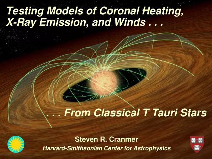
Testing Models of Coronal Heating, X-Ray Emission, and Winds. . . . From Classical T Tauri Stars. Steven R. Cranmer Harvard-Smithsonian Center for Astrophysics. Outline: Brief overview of T Tauri star & solar activity Impact-driven turbulence: a plausible chain of events?

E N D
Testing Models of Coronal Heating, X-Ray Emission, and Winds . . . . . . From Classical T Tauri Stars Steven R. CranmerHarvard-Smithsonian Center for Astrophysics
Outline: • Brief overview of T Tauri star & solar activity • Impact-driven turbulence: a plausible chain of events? • Testing the hypothesis: Testing Models of Coronal Heating, X-Ray Emission, and Winds . . . • Accretion shocks • Coronal loops • Stellar winds . . . From Classical T Tauri Stars Steven R. CranmerHarvard-Smithsonian Center for Astrophysics
T Tauri stars: complex geometry & activity • T Tauri stars show signatures of disk accretion, “magnetospheric accretion streams,” an X-ray corona, and polar (?) outflowsfrom some combination of star & disk. • Nearly every observational diagnostic varies in time, sometimes with stellar rotation, but often more irregularly. (Romanova et al. 2007) (Rucinski et al. 2008) (Matt & Pudritz 2005, 2008)
Context from the Sun’s corona & wind • Photospheric flux tubes are shaken by an observed spectrum of convective motions. • Alfvén waves propagate along the field, and partly reflect back down (non-WKB). • Nonlinear couplings allow MHD turbulence to occur: cascade produces dissipation. Closed field lines experience strong turbulent heating Open field lines see weaker turbulent heating & “wave pressure” acceleration
Ansatz: accretion stream impacts make waves • The impact of inhomogeneous “clumps” on the stellar surface can generate MHD waves that propagate out horizontally and enhance existing surface turbulence. • Scheurwater & Kuijpers (1988) computed the fraction of a blob’s kinetic energy that is released in the form of far-field wave energy. • Cranmer (2008, 2009) estimated wave power emitted by a steady stream of blobs. similar to solar flare generated Moreton/EUV waves?
Testing the ansatz… with real stars • Classical T Tauri stars in the Taurus-Auriga star forming region are well-observed: AA Tau BP Tau CY Tau DE Tau DF Tau DK Tau DN Tau DO Tau DS Tau GG Tau GI Tau GM Aur HN Tau UY Aur • Cranmer (2009) used two independent sets of M*, L*, R*, ages, & accretion rates, from Hartigan et al. (1995) and Hartmann et al. (1998). • Accretion spot “filling factors” δ taken from Calvet & Gullbring (1998) measurements of Balmer & Paschen continua → accretion energy fluxes & areas. • Surface magnetic field strengths B* for 10/14 stars taken from Johns-Krull (2007) measurements of Ti-line Zeeman broadening; other 4 fromempirical <B*/Bequi>.
Start with the simplest geometry • Königl (1991) showed how inner-disk edge can scale with stellar parameters: • Measured filling factor δ gives router, as well as size of blobs at stellar surface. • Assume ballistic (free-fall) velocity to compute ram pressure; this gives ρshock/ρphoto. • The streams are inhomogeneous: • Need to assume “contrast:” ρblob/<ρ> ≈ 3. • This allows us to compute: L. Hartmann, lecture notes N (number of flux tubes impacting the star) Δt (inter-blob intermittency time)
Accretion shock models • Temporarily ignoring the existence of “blobs” allows a straightforward 1D calculation of time-steady shock conditions & the post-shock cooling zone. • Typical post-shock conditions: log Te ~ 5–6, log ne ~ 13.5–15 • Cranmer (2009) synthesized X-ray luminosities: ROSAT (PSPC), XMM (EPIC-pn).
Results: accretion shock X-rays • Blah…
Coronal loops: MHD turbulent heating • Cranmer (2009) modeled equatorial zones of T Tauri stars as a collection of closed loops, energized by “footpoint shaking” (via blob-impact surface turbulence). • Coronal loops are always in motion, with waves & bulk flows propagating back and forth along the field lines. • Traditional Kolmogorov (1941) dissipation must be modified because counter-propagating Alfvén waves aren’t simple “eddies.” n =0 (Kolmogorov), 3/2 (Gomez), 5/3 (Kraichnan), 2 (van Ballegooijen), f(VA/veddy) (Rappazzo) • T, ρalong loops computed via Martens (2010) scaling laws: log Tmax ~ 6.6–7.
Stellar winds from polar regions • The Scheurwater & Kuijpers (1988) wave generation mechanism allows us to compute the Alfvén wave velocity amplitude on the “polar cap” photosphere . . . • Waves propagate up the flux tubes & accelerate the flow via “wave pressure.” • If densities are low, waves cascade and dissipate, giving rise to T > 106 K. • If densities are high, radiative cooling is too strong to allow coronal heating. • Cranmer (2009) used the “cold” wave-driven wind theory of Holzer et al. (1983) to solve for stellar mass loss rates. photosph. sound speed ( ) 1 solar mass model v┴from accretion impacts v┴from interior convection
Results: wind mass loss rates O I 6300 blueshifts (yellow) (Hartigan et al. 1995) Model predictions O I 6300 blueshifts (yellow) (Hartigan et al. 1995) Model predictions
Conclusions • Insights from solar MHD have led to models that demonstrate how the accretion energy can contribute significantly to driving T Tauri outflows & X-ray emission. . • Is Mwind enough to solve the T Tauri angular momentum problem? • Why do (non-accreting) weak-lined T Tauri stars show stronger X-rays? • More realistic models must include: (1) more complex magnetic fields, and (2) the effects of rapid rotation on convective dynamo “activity.” Cohen et al. (2010) Brown et al. (2010) For more information: http://www.cfa.harvard.edu/~scranmer/
How did we get here? • The Young Sun: • Kelvin-Helmholz contraction: An ISMcloud fragment becomes a “protostar;” gravitational energy is converted to heat. • Hayashi track: protostar reaches approx. hydrostatic equilibrium, but slower gravitational contraction continues. Observed as the T Tauri phase. • Henyey track: Tcore reaches ~107 K and hydrogen burning begins to dominate → ZAMS.
Mass loss: where does it originate? • YSOs (Class I & II) show jets that remain collimated far away (AU →pc!) from the central star. Outflows anchored in disk? • However, EUV emission lines and He I 10830 Å P Cygni profiles indicate that blueshifted outflows are close to the star. • Stellar winds & disk winds may co-exist. (Ferreira et al. 2006)
Mass loss • Mwind is obtained from signatures of blueshifted opacity (~few 100 km/s). • For example . . . • Forbidden emission lines [O I], [Si II], [N II], [Fe II] (Hartigan et al. 1995) • P Cygni absorption trough of He I 10830 (chromospheric diagnostic): M acc Hartigan et al. (1995) TW Hya: Batalha et al. (2002) Dupree et al. (2005)
Ansatz: accretion stream impacts make waves similar to solar flare generated Moreton/EUV waves?
More solar precedents • Solar flares and coronal mass ejections (CMEs) can set off wave-like “tsunamis” on the solar surface . . . • Moreton waves propagate mainly as chromospheric Hα variations, at speeds of 400 to 2000 km/s and last for only ~10 min. Fast-mode MHD shock? • “EIT waves” show up in EUV images, are slower (25–450 km/s), and can traverse the whole Sun over a few hours. Slow-mode MHD soliton?? NSO press release (Dec. 7, 2006) Wu et al. (2001)
Properties of accretion streams • Königl (1991) showed how inner-disk edge scales with stellar parameters: • Dipole geometry gives δ (fraction of stellar surface filled by columns) and rblob. • Assume ballistic (free-fall) velocity to compute ram-pressure balance; gives ρshock / ρphoto. • The streams are inhomogeneous: • Need to assume “contrast:” ρblob / <ρ> ≈ 3. • This allows us to compute: L. Hartmann, lecture notes N (number of flux tubes impacting the star) Δt (inter-blob intermittency time)
Accretion-driven T Tauri winds • Results: wind mass loss rate increases ~similarly with the accretion rate. • For high enough densities, radiative cooling “kills” the coronal heating!
Cool-star rotation → mass loss? • There is a well-known “rotation-age-activity” relationship that shows how coronal heating weakens as young (solar-type) stars age and spin down (Noyes et al. 1984). • X-ray fluxes also scale with mean magnetic fields of dwarf stars (Saar 2001). • For solar-type stars, mass loss rates scale with coronal heating & field strength. • What’s the cause? With more rapid rotation, • Convection may get more vigorous (Brown et al. 2008, 2010) ? • Lower effective gravity allows more magnetic flux to emerge, thus giving a higher filling factor of flux tubes on the surface (Holzwarth 2007)? (Mamajek 2009)
Evolved cool stars: RG, HB, AGB, Mira • The extended atmospheres of red giants and supergiants are likely to be cool (i.e., not highly ionized or “coronal” like the Sun). • High-luminosity: radiative driving... of dust? • Shock-heated “calorispheres”(Willson 2000) ? • Numerical models show that pulsations couple with radiation/dust formation to be able to drive mass loss rates up to 10 –5 to 10 –4Ms/yr. (Struck et al. 2004)
The extended “solar atmosphere” Everywhere one looks, the plasma is “out of equilibrium”
The solar corona • Plasma at 106 K emits most of its spectrum in the UV and X-ray. • The “coronal heating problem” remains unsolved . . . . Coronal hole (open) “Quiet” regions Active regions
heat conduction radiation losses 5 2 — ρvkT What sets the Sun’s mass loss? • Coronal heating must be ultimately responsible. • Hammer (1982) & Withbroe (1988) suggested a steady-state energy balance: • Only a fraction of total coronal heat flux conducts down, but in general, we expect something close to . . . along open flux tubes!
Wang et al. (2000) Solar wind: connectivity to the corona • 1958:Eugene Parkerproposed that the hot corona provides enough gas pressure to counteract gravity and accelerate a “solar wind.” 1962:Mariner 2 saw it! • High-speed wind (600–800 km/s): strong connections to largest coronal holes. • Low-speed wind (300-500 km/s): no agreement on full range of source regions in the corona: “helmet streamers,” small coronal holes, active regions . . . Fisk (2005)
In situ fluctuations & turbulence • Fourier transform of B(t), v(t), etc., into frequency: f -1 “energy containing range” f -5/3 “inertial range” The inertial range is a “pipeline” for transporting magnetic energy from the large scales to the small scales, where dissipation can occur. Magnetic Power f -3“dissipation range” few hours 0.5 Hz
What processes drive solar wind acceleration? Two broad paradigms have emerged . . . • Wave/Turbulence-Driven (WTD) models, in which flux tubes “stay open” • Reconnection/Loop-Opening (RLO) models, in which mass/energy is injected from closed-field regions. vs. • There’s a natural appeal to the RLO idea, since only a small fraction of the Sun’s magnetic flux is open. Open flux tubes are always near closed loops! • The “magnetic carpet” is continuously churning. • Open-field regions show frequent coronal jets (SOHO, Hinode/XRT).
Waves & turbulence in open flux tubes • Photospheric flux tubes are shaken by an observed spectrum of horizontal motions. • Alfvén waves propagate along the field, and partly reflect back down (non-WKB). • Nonlinear couplings allow a (mainly perpendicular) cascade, terminated by damping. (Heinemann & Olbert 1980; Hollweg 1981, 1986; Velli 1993; Matthaeus et al. 1999; Dmitruk et al. 2001, 2002; Cranmer & van Ballegooijen 2003, 2005; Verdini et al. 2005; Oughton et al. 2006; many others)
Waves & turbulence in the photosphere • Helioseismology: direct probe of wave oscillations below the photosphere (via modulations in intensity & Doppler velocity) • How much of that wave energy “leaks” up into the corona & solar wind? Still a topic of vigorous debate! • Measuring horizontal motions of magnetic flux tubes is more difficult . . . but may be more important? splitting/merging torsion 0.1″ longitudinal flow/wave bending (kink-mode wave)
Dissipation of MHD turbulence • Standard nonlinear terms have a cascade energy flux that gives phenomenologically simple heating: • We used a generalization based on unequal wave fluxes along the field . . . (“cascade efficiency”) Z– Z+ • n = 1: usual “golden rule;” we also tried n = 2. • Caution: this is an order-of-magnitude scaling! (e.g., Pouquet et al. 1976; Dobrowolny et al. 1980; Zhou & Matthaeus 1990; Hossain et al. 1995; Dmitruk et al. 2002; Oughton et al. 2006) Z–
The solar wind acceleration debate • What determines how much energy and momentum goes into the solar wind? • Waves & turbulence input from below? • Reconnection & mass input from loops? vs. • Cranmer et al. (2007) explored the wave/turbulence paradigm with self-consistent 1D models of individual open flux tubes. • Boundary conditions imposed only at the photosphere (no arbitrary “heating functions”). • Wind acceleration determined by a combination of magnetic flux-tube geometry, gradual Alfvén-wave reflection, and outward wave pressure.
Understanding physics reaps practical benefits 3D global MHD models Real-time “space weather” predictions? Self-consistent WTD models Z– Z+ Z–