Advanced Techniques for Visibility Optimization in 3D Graphics

1. Visibility Culling Markus Hadwiger & Andreas Varga

2. Basics • Hierarchical Subdivision • Hierarchical Bounding Boxes • Octrees • K-D Trees ( K-Dimensional Space) • BSP Trees ( Binary Space Partition ) • Potentially Visible Sets (PVS)

3. Hierarchical Bounding Box (HS) • Construct a bounding box for each object • Merge nearby bounding box into bigger ones • Not very structured and systematic • Perform well for certain viewpoint • Shortcomings: • Highly dependent on the given scene(worse: on the actual viewpoint) • Unpredictable not very useful !

4. Hierarchical Bounding Box Example (HS) WORLD ROLLERCOASTER CAR #2 CAR #1 GUY_BAD GUY_BAD GUN GUY_BAD

5. Octrees (HS) • Each node of and octree has form one to eight children if it is an internal node; otherwise it is a leaf node • Culling against the viewing frustum • Shortcomings of regular subdivision • Efficiently problem (inflexible) • Depend on the location of each polygon • The two dimensional version of an octree is called quadtree

6. Octrees Example (HS)

7. K-D Trees2/2(HS) • Hierarchically subdivide n-dimensional space • A binary tree • partitioning space into two halfspaces at each level • two equal-sized partitions is not necessary (Octrees) • Always done axial • A separating hyperplane can depend on actual data • Balance of binary tree • One halfspace contains the same number of objects as the other halfspace

8. K-D Trees Example 1/2(HS) 4 6 1 10 8 11 2 3 3 13 2 4 5 6 7 12 9 8 9 10 11 12 13 5 1 7

9. K-D Trees Example 2/2(HS)

10. BSP Trees6(HS) • Generalization of k-D trees • Space is subdivided along arbitrarily oriented hyperlpanes • Subdivision of space into two halfspace at each step • Produces a binary tree • Internal node corresponds to the partitioning hyperplane • Leaf nodes are empty halfspaces • Exact visibility determination for arbitrary viewpoint • For entirely static polygonal scenes • Can be precalculated onceand traversal at run time witharbitrary viewpoint

11. BSP Trees Example 1(HS) 2 3 1 1 4 5 6

12. BSP Trees Example 2(HS) 1 2 front 3 1 4a 2 4b 5 6

13. BSP Trees Example 3(HS) 1 2 front back 3 1 4a 2 3 4b 5 6

14. BSP Trees Example 4(HS) 1 2 front back 3 1 4a 2 3 4b front back 5 6 4a 4b

15. BSP Trees Example 5(HS) 1 2 front back 3 1 4a 2 3 4b front back front 5 6 4a 5 4b front 6

16. BSP Trees Example 6(HS) 1 2 V1 front back 3 1 2 3 4 front back front 5 6 4a 5 4b V2 front 6 • The painting order from V1: 3, 5, 1, 4b, 2, 6, 4a • The painting order from V2: 3, 5, 1, 4b, 2, 4a, 6 • We got correct picture of who is behind whom no matter where we were looking from.

17. BSP Trees Example 6(HS)

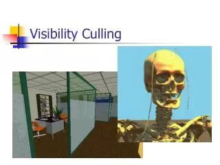
18. Cell-Portals • Assume the world can be broken into cells • Simple shapes • Rooms in a building, for instance • Defineportalsto be the transparent boundaries between cells • Doorways between rooms, windows, etc • In a world like this, can determine exactly which parts of which rooms are visible • Then render visible rooms plus contents

19. Cell-Portals Example A B A B • －Portals can be one way (directed edges) • －Graph is normally stored in adjacency list format • －Each cell stores the edges (portals) out of it C D C D E F E F －Node are cells, edges are portals－K-D trees and BSP trees are used to generate the cell structure and find neighbors and portals

20. Cell and Portal Visibility • Keep track of which cell the viewer is in • Somehow walk the graph to enumerate all the visible regions • Can be done as a preprocess to identify the potentially visible set (PVS) for each cell • Cell-to-region visibility, or cell-to-object visibility • Can be done at run-time for a more accurate visible set • Start at the known viewer location • Eye-to-region or Eye-to-cell visibility • Trade-offis between time spent rendering more than is necessary vs. time spent computing a smaller set • Depends on the environment, such as the size of cells, density of objects, …

21. Potentially Visible Sets (PVS) • PVS: The set of cells/regions/objects/polygons that can be seen from a particular cell • Generally, choose to identify objects that can be seen • Trade-off is memory consumption vs. accurate visibility • Computed as a pre-process • Have to have a strategy to manage dynamic objects • Used in various ways: • As the only visibility computation - render everything in the PVS for the viewer’s current cell • As a first step - identify regions that are of interest for more accurate run-time algorithms

22. Cell-to-Cell PVS • Cell A is in cell B’s PVS if there exist a stabbing line that originates on a portal of B and reaches a portal of A • A stabbing line is a line segment intersecting only portals • Neighbor cells are trivially in the PVS I J PVS for I contains: B, C, E, F, H, J F H D B E C G A

23. Finding Stabbing Lines R L L • In 2D, have to find a line that separates the left edges of the portals from the right edges • In 3D, more complex because portals are now a sequence of arbitrarily aligned polygons • Put rectangular bounding boxes around each portal and stab those R R L R L

24. Stab Trees • A stab tree indicates: • The PVS for a cell • The portal sequences to get from one to the other • Used in further visibility processing • Restricts number of cells/portals that must be looked at A A B A/C C C/E C/D2 C D C/D1 E D D D/F F E F

25. Run-Time Visibility • PVS approaches are entirely pre-processing • At run time, just render PVS • Better results can be obtained with a little run-time processing • Sometimes guided by PVS • It appears that most games don’t bother, the trade-off favors pre-processed visibility and over-rendering • At run time the viewer’s location is known, hence Eye-to-Region visibility

26. Eye-to-Cell • Recall that finding stabbing lines involved finding a line that passed through all the portals • The viewer adds some constraints: • The stabbing line must pass through the eye • It must be inside the view frustum • The resulting problem is still reasonably fast to solve • Results in knowledge of which cells are visible from the eye • Use the stab tree from the PVS computation to avoid wasting effort • Further optimization is to keep reducing the view frustum as it passes through each portal, which leads us to…

27. Eye-to-Region Visibility • Define a procedure : • Takes a view frustum and a cell • Viewer not necessarily in the cell • Draws the contents of the cell that are in the frustum • For each portal out of the cell, clips the frustum to that portal and recurs with the new frustum and the cell beyond the portal • Make sure not to go to the cell you entered • Start in the cell containing the viewer, with the full viewing frustum • Stop when no more portals intersect the view frustum

28. Eye-to-Region Example View

29. Eye-to-Region Example View

30. Eye-to-Region Example View

31. Eye-to-Region Example View

32. Eye-to-Region Example View

33. Eye-to-Region Example View View

34. Eye-to-Region Example View

35. Non-Invasive Interactive Visualization of Architectural Environments Christopher Niederauer U.C. Santa Barbara Mike Houston Stanford University Maneesh Agrawala Microsoft Research Greg Humphreys University of Virginia

36. Problem • Environments of video game are vast and tend to be densely occluded. • Most 3D model viewing application lack the ability to simultaneously display the interior spaces and the external structure of the environment.

37. Motivation Arcball style manipulator Walkthrough ArcBall [Shoemake 1992] [Teller 1992] Can’t see overall interior/exterior structure!

38. Motivation Quake III[Id Software c. 2002] The occlusions make it impossible to see all the action at once!

39. The Idea • Exploded view • just below the ceilings • Non-Invasive[Mohr 2001] • without modification • use Chromium [Humphreys et al. 2002] Overall structure is visible!

40. Geometric Analysis Rendering Floor Gather Data Find Splits Composite … Floor How It’s Done • Example Architecture: Soda Hall • Geometric Analysis(once) • Rendering(every frame) OpenGL Stream

41. Gather Architectural Data • Intercept the OpenGL stream • Find downward facing polygons • Requires up-vector 1 up 2 3 polygon normal = (v2-v1)x(v3-v2) • Compute theheight of downward facing polygon 1 height = v1‧upVector

42. Gather Architectural Data Height Ceiling Area • Create Histogram 942 766 606 446 286 126 Soda Hall Side Profile Geometric Analysis Rendering Floor OpenGL Stream Gather Data Find Splits Composite … Floor

43. Find Splitting Heights Geometric Analysis Rendering Floor OpenGL Stream Gather Data Find Splits Composite … Floor

44. Offset Ceiling Heights

45. Offset Ceiling Heights

46. NumSplits Player Height Up Vector Geometric Analysis Rendering Geometric Analysis Floor Gather Data Find Splits OpenGL Stream … Composite Floor Find Downward Facing Polygons Table MappingHeight to Surface Area Find Split Heights List of Split Height

47. Rendering • Multiple Playback (Once per Floor) • Viewpoint Control • Clipping Planes • Translate along Up Vector Geometric Analysis Rendering Floor OpenGL Stream Gather Data Find Splits Composite … Floor

48. GeometricAnalysis Rendering OriginalApplicationOpenGL List of SplitHeights SeparationDistance Viewpoint Set ViewpointClip Plans &Translation NumSplits Passes of Modified OpenGL NumSplits Passes ofOriginal OpenGL NumSplits … Exploded viewvisualization MultiplePlayback MultipassComposite Set ViewpointClip Plans &Translation

49. Cluster Speedup Complete Model Floor 2 Floor 3 Floor 1 800 MHz Pentium III Xeon processorNVIDIA GeForce4 graphics accelerator Composite

50. Soda Hall Trackball Walkthrough