Download
1 / 78
930 likes | 1.57k Views
PPARC Advanced Summer School in Solar Physics. Structure of the solar corona. Ramón Oliver Universitat de les Illes Balears. Purpose. An hour and a half worth of … … some basic observational facts about the solar corona and … some basic understanding about the solar corona

E N D
PPARC Advanced Summer School in Solar Physics Structure of the solar corona Ramón Oliver Universitat de les Illes Balears
Purpose • An hour and a half worth of … • … some basic observational facts about the solar corona and • … some basic understanding about the solar corona • Re-examination of familiar concepts • Robertus e-mail message: “… I usually give choco or beer or a poster or a nice picture about the Sun …”
Outline • Large-scale structure and physical conditions of the corona • Small-scale structure: active regions & loops • The dynamic corona • Large-scale structure and physical conditions of the corona • Small-scale structure: active regions & loops • The dynamic corona
Solar eclipse totality • Total solar eclipses gave the first glimpse of the solar corona (106 times dimmer than photosphere) • Warning: beware of image processing. During an eclipse, the corona is 100 times brighter at solar limb than at 1 R☉ height
Large-scale structures • Two types of structures: • Thin plumes near the poles • Long streamers near the equator How persistent is this structuring? Just wait!
Large-scale structures • Eclipse (blue-ish) + LASCO C2 image (orange-ish) • LASCO C2 FOV→ 2-6 R☉ • Streamers extend out many solar radii • Shape of coronachanges in time(Δt ≈ 18 months) • Polar plumes? • Note projection onthe plane of the sky • Many superposedstructures
The white light corona (K-corona) • Coronal emission in eclipses and with coronagraphs consists of photospheric radiation scattered off coronal electrons • This process is equivalent to that responsible for the halo around a street lamp in the fog A photon is deflectedby an electron A few photons are deflected ~ 90° • By the way… there are free electrons in the corona
Coronal density • Observed brightness + theory of Thomson scattering used in the first determinations of coronal density→ ne~ 107-109 cm-3 • 106-108 times less dense than the photospheric gas • Less dense than best vacuum in Earth’s laboratories • Variation with height: ne decreases with h ⇨ cause of reduction of brightness with height
Coronal temperature • Corona emits its own light (scattering is not emission!) • Slitless spectrum during eclipse • Chromosphere not completely occulted ⇨ spectral “lines” HeI Hβ Hγ Hδ CaII Hα • Slitless spectrum of corona during eclipse • Green, red and yellow coronal lines (5303 Å, 6374 Å, 5694 Å) • Emission from Fe+13, Fe+9 and Ca+14 → FeXIV, FeX, CaXV • Known as E-corona (vs. the K-corona we see in eclipses)
Coronal temperature • Presence of highly ionised atoms possible because of high coronal temperature • Ionisation equilibrium in corona → balance between • Remember: temperature is a measure of average kinetic energy of gas particles • High temperature → large electron velocities → energetic collisions → ionisation collisional ionisation ⇔ recombination
Coronal temperature • Ionisation balance calculations lead to fractional ion abundances as a function of temperature: • Fe+9 most abundant for T ~ 106 K • Fe+13 most abundant for T ~ 2×10⁶ K • Ca+14 most abundant for T ~ 4×10⁶ K • Corona is suprathermal and multi-temperature
Suprathermal corona • The temperature grows from ~ 5800 K in the photosphere to ~ 106 K in the corona • This is unexpected: the atmosphere does not show the outward temperature decrease of the solar interior (caused by flow of atomic fusion energy) • Convective motions below the surface may be the cause of chromospheric heating (but not coronal heating) • Meet “THE CORONAL HEATING PROBLEM” • Solution: unknown, but most probably MAGNETIC • Talks “Coronal heating: observations” & “Coronal heating: theory”
Multi-temperature corona • Existence of the green, red and yellow coronal lines implies corona is not isothermal • Corona emits in a multitude of lines outside the visible spectrum (mostly EUV & soft X-rays → SXR) • Some spectral lines used by EIT or TRACE and temperature sensitivity
Multi-temperature corona • Simultaneous images with EIT coronal filters 1 MK 2-2.5 MK 1.5 MK
Multi-temperature corona • Yohkoh soft X-ray telescope (SXT) records SXR emission of plasma at 2-5 MK • Comparison between TRACE (171 Å) and SXT images; SXT has poorer spatially resolution ⇨ different appearance of structures Size of FOV 700 Mm × 350 Mm
Multi-temperature corona • All over the corona gas elements at widely different temperatures are close neighbours • How dynamic is this situation? Do these elements interchange heat until temperature equilibrium is achieved? More about this later
Coronal composition • The huge temperature leads to full ionisation of H and partial ionisation of He and metals • Remember: collisions responsible for ionisation • Thus, the corona is made of a mixture of electrons and ions • Protons and electrons are the most abundant • The coronal gas is in a (partially ionised) PLASMA state • Interacts with (electro)magnetic fields • Can be treated as a fluid • Magnetohydrodynamic approximation
Coronal composition • Abundances in the coronal gas is similar to photospheric ~ 91% hydrogen atoms (fully ionised) ~ 8.9% helium atoms ~ 0.1% metals • But there are some differences: different ionisation states A few elements are more abundant than in photosphere; He is less abundant
Origin of coronal structuring • Classical modelling of the stellar interiors and atmospheres based on gravitational stratification⇨ balance of pressure gradient and gravity forces • Consequence: physical parameters vary ONLY in the radial direction, NO horizontal structures • Streamers and plumes should not exist! • Some force is shaping the coronal gas… … MAGNETISM • The magnetic field is the dominant organising force in the low corona
Solar magnetism • A few keywords: • Convective motions, magnetic field generation in the tachocline & magnetic flux emergence • Talks “Structure of the Sun: the solar interior” & “Dynamo theory” • Photospheric magnetic fields: spatial intermittency, i.e. 100 G to kG fields very unevenly distributed • Talk: “The structure of the lower solar atmosphere” • Coronal structure is direct consequence of shape of magnetic fields emerging through photosphere
Photospheric magnetism • Magnetogram → distribution of photospheric magnetic flux • White/black → strong magnetic field • Grey → weak/no mag. field • Large-scale structures dominate, but intense flux concentrations present at ≲ 1 Mm scales (i.e. spatial resolution limit ⇨ maybe flux tubes are thinner than 1 Mm)
Magnetic field structure • Flux tubes expand in chromosphere and transition region and become space-filling in corona • Magnetic field lines connect two opposite photospheric polarities Large flux concentrations Smaller flux concentrations Magnetogram: green instead of grey
Coronal magnetic structure • Field lines often close at very large distance • Magnetic field lines in the corona can be: • Closed: connecting two opposite photospheric polarities • Open: length of field lines is infinite in practice Coronal magnetic fieldline configuration Magnetogram: yellow & orangeinstead of white & grey
Coronal structure • Coronal magnetic topology based on magnetogram data for 03/17/2006 & used to PREDICT magnetic configuration on 03/26/2006 (total eclipse!) • Open field lines in polar regions → polar plumes • Closed field lines in equatorial region → streamers Plasma maps out coronal magnetic field geometry
Coronal structure • The shape of magnetic field lines reflects itself in the structures of the corona; comparison with LASCO C2 • LASCO image: continuation of streamers and some polar plumes
Coronal structure • And now LASCO C2 and C3 • LASCO C3 FOV→ 4-30 R☉ • Streamers extendradially many R☉
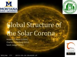
Coronal structure • High EUV emission occurs above pairs of strong photospheric magnetic flux →ACTIVE REGIONS • Emergence of fresh magnetic flux gives rise to a host of dynamic phenomena 1.5 MK 2-2.5 MK
Coronal structure • EUV & white light corona (LASCO C2) • Streamers aboveactive regions CME 2-2.5 MK 1.5 MK 1 MK
Coronal structure • Clockwise: 171 Å, 195 Å, 284 Å, Yohkoh SXR & magnetogram • Big image: superposition of the three TRACE EUV images • Corona composed of: • Active regions: the brightest elements, from 1 to 5 MK; closed magnetic fields • Coronal holes: clearly dark in SXR; open magnetic field lines, usually near the poles • Quiet Sun: areas outside active regions & coronal holes; closed field lines; not quiet at all!!
Frozen flux theorem • Because of the very large coronal length-scales, the MHD induction equation dictates that the magnetic flux is “frozen-in” to the fluid • Field lines are like elastic bands • A plasma element moving across a magnetic field is tied to field lines and so drags them • Plasma elements cannot crossthe limits of magnetic flux tubes • Plasma elements can only freely move ALONG field lines
Density and temperature (once more) • Active regions have the largest n and T • n ~ 108-109 cm-3, T ~ 2-6 MK • Activity ⇨ injection of chromospheric material and heating • Closed magnetic topology ⇨ effective plasma confinement • Quiet sun → smaller density and temperature • n ~ 1-2×108 cm-3, T ~ 1-2 MK • Closed magnetic field, but less activity ⇨ reduced mass injection, reduced heat input rate • Coronal holes → rarer and cooler • n ~ 0.5-1×108 cm-3, T ≲ 1 MK • Open field configuration ⇨ particles escape more easily
Section summary • Coronal magnetic fields are organised in open and closed configurations • Open fields prevail in the polar regions ⇨ coronal holes & polar plumes • Closed fields connect intense photospheric magnetic pairs ⇨ active regions & streamers • Closed fields (e.g. between neighbouring active regions) ⇨ “quiet Sun” • Plasma in corona is suprathermal & multi-temperature • Hot plasma emits mostly in EUV and X-ray lines
Outline • Large-scale structure and physical conditions of the corona • Small-scale structure: active regions & loops • The dynamic corona
Active regions • An active region is a portion of the corona overlying two opposite strong magnetic polarities visible here as a sunspot pair • Active regions occupy only a fraction of the Sun’s surface area, but harbour most ofcoronal activity • Flares, CMEs, plasmaheating, flows, waves, etc.
Active regions • Origin of this activity • Magnetic flux emergence, magnetic flux cancellation, magnetic reconfiguration, magnetic reconnection • Consequence of activity →chromospheric upflows inject material in the corona • Many loops filled with hot, dense plasma • Emission in EUV & SXR Composite of TRACE 171 Å images
Active regions & loops • Close look at an active region using TRACE: • three dimensional structure extending to great heights • complex arrangement of tubular arches (loops) Loops merge large and small scales: length and thickness (~ 1 Mm), respectively Are loops resolved by TRACE observations (0.5” spatial resolution)? Loops delineate path of magnetic fields
Ubiquitous loops? • Despite the omnipresence of loop structures in coronal EUV images, loops are actually relatively rare • If many more loops were present in a given area, then isolated loops would not be so clearly visible
Loop emission • Coronal loops are detected because: • They have the right temperature to emit in the filter passband • Emitted intensity roughly proportional to ne2⇨ loops are visible only if they are dense enough
Loop thickness • Why are loops so thin? • Small loop widths are a consequence of the transverse size of photospheric magnetic fields • But then, why doesn’t the loop material spread in the transverse direction? • Because of frozen flux theorem, plasma elements are confined to the limits of the magnetic flux tube and can only freely move ALONG the loop
Loops & equilibrium • We know very well that some loops are dynamic objects • However, why not assume some of them are in some sort of equilibrium? • Let us introduce some theoretical concepts • Hydrostatic equilibrium • Magnetohydrostatic equilibrium • Robertus e-mail message: “… do not have too much maths, but SOME maths can be delivered for those interested in the theory…” → Here we go!
Hydrostatic equilibrium • Let us consider a gas in hydrostatic equilibrium ⇨ no time variations + balance of –∇p and ρg –∇p + ρg = 0 • Assume only dependence with height (z = r–R☉) –dp/dz – ρg = 0 • Assume ideal gas law → p = ρRT/ξ • ξ comes from adding together the pressure of electrons, protons & ions • ξ = 0.5 in a fully ionised H plasma • ξ~ 0.635 in corona (mostly because of 4He) • Assume uniform temperature (really?) • Gravitational acceleration: g = g☉(R☉/r)2(g☉=274 m s-1)
Hydrostatic equilibrium • Neglect radial variation of g (so take g = g☉) • p, ρdecrease exponentially with height p(z) = p0exp(–z/Λ), Λ = RT/ξg☉ • Λ is the gravitational scale-height:Λ = 47.7 T6 Mm T6=T/106 K • If radial variation of g not neglected p(z) = p0exp[–z/Λ(1+z/R☉)] • Some remarks: • p ~ const. for small variations of z or large T • Close to surface z ≪ R☉ and the two expressions agree • For T = 1 MK and z = 100 Mm the exponential approximation underestimates the pressure by 23%
Magnetohydrostatic equilibrium • A magnetic field B exerts a force j×B per unit volume on a plasma element • j = ∇×B/μ(from Ampere’s law) is the current density • j×B is called the Lorentz force • Comes from the force qv×B on a charge q with velocity v • The force balance equation now is–∇p + ρg + j×B= 0 • Does the equilibrium solution differ too much from the hydrostatic one?
Magnetohydrostatic equilibrium • Scalar product by B (⇨ we follow the loop field line)–B⋅∇p + ρB⋅g = 0 ⇨ –B dp/ds – B ρg cosθ = 0 ⇨ dp/dz + ρg = 0 • Same equation of hydrostatic case • Same vertical dependence of densityand pressure • BUT each loop can have its own T⇨ its own Λ⇨ different loops maybehave in a different manner • Loops are like mini-atmospheres
Are loops in hydrostatic equilibrium? • TRACE image in 171 Å filter • Sensitive to 106 K temperature • If hydrostatic equilibrium ⇨n(z) = n0exp(–z/Λ) with Λ~ 47.7 Mm • The line intensity is proportional to n2⇨I(z) = I0exp(–2z/Λ) ⇨ scale-height is Λ / 2 ~ 25 Mm • Intensity decreases by almost 40% every 25 Mm • Is this what we observe? • Very probably not
Are loops in hydrostatic equilibrium? • Analysis of 40 loops, measure scale-height (Λm) • Loops selected if intensity contrast is significant along their whole length • But, suppose a long loop is in hydrostatic equilibrium → intensity decreases substantially from bottom to top → loop is discarded ! • Long loops in hydrostatic equilibrium cannot be detected with this selection criterion
Are loops in hydrostatic equilibrium? • Results: only a few loops have Λm~ Λ, all other loops are not in (magneto)hydrostatic equilibrium No long loops in hydrostatic equilibrium found (as expected) Λm/Λ Moreover, many loops not in hydrostatic equilibrium • What is wrong? Our assumption of force balance • Dynamics (flows, waves, …), but also energetics (heating & cooling ) must be taken into account
Are loops in hydrostatic equilibrium? • Forces required to lift up the large quantities of plasma illustrated by simulated image based on hydrostatic balance How active region looks like How it would look like if in hydrostatic equilibrium
Plasma beta • Relative importance of forces through dimensional analysis: |–∇p| / |ρg| ~ p/L / ρg = Λ/L • Pressure force dominates over gravity on short vertical distances (Λ/L≫1); gravity important in high structures (Λ/L≪1) • Lorentz force j×B = 1/μ(∇×B)×B: |–∇p| / |j×B| ~ p/L / (B2/μL) ~ 2μp/B2 = β • Magnetically dominated plasma for β≪1 • Lorentz force:j×B = 1/μ(∇×B)×B = 1/μ(B⋅∇)B– ∇(B2/2μ)1/μ(B⋅∇)B → magnetic tension force –∇(B2/2μ) → gradient of magnetic pressure
Coronal magnetic field modelling • Little observational information about coronal magnetic field ⇨ numerical modelling • The solar corona is usually described as a low-β plasma • The magnetic Lorentz force then is said to shape the coronal plasma • The influence of gravity is neglected (is this realistic?) • Force balance equation reduces to j×B = 0 ! • j = 0 ⇨ ∇×B = 0 potential solution • j ≠ 0 ⇨ (∇×B)×B = 0 force-free solution • Partial differential equations for B solved; boundary conditions = photospheric magnetic field distribution • Real b.c. should be chromospheric magnetic field