Download
1 / 14
140 likes | 274 Views
Vertical Resolution of HIRDLS Temperature Data John Barnett HIRDLS Science Team Meeting January 30-31 2008. Comparisons between COSMIC GPS radio occultation data and HIRDLS

E N D
Vertical Resolution of HIRDLS Temperature Data John Barnett HIRDLS Science Team Meeting January 30-31 2008
Comparisons between COSMIC GPS radio occultation data and HIRDLS These profiles used HIRDLS profiles within 0.75 deg (great circle), i.e. 83.3 km and 500 sec of time of the COSMIC profile. Sometimes 2 (possibly 3) HIRDLS profiles matched this criterion, in which case they were averaged together. • Two methods of comparison were used: • Subtract a smoothed profile (this is equivalent to a high pass filter) then intercorrelate HIRDLS, COSMIC and GMAO. Each used its own smoothed profile. Results for a 0.5 pressure scale heights full width at half height filter are shown first, then for a 0.8 FWHH filter. • Fourier analysis over the range 2.2-5.7 scale heights, after fitting a parabola to remove the background, and apodizing. 0.5 scaleheights = approx 3.5 km
Main aim is to validate HIRDLS vertical resolution. Fitted smooth (10 km wide filter) profiles to both then analysed deviations over range 2.0 to 4.75 scale heights. The HIRDLS retrieval is climatology in the mid and lower troposphere, but should be accurate up to about 60 km (8 pressure scale heights). COSMIC data are generally thought to be accurate up to 30-35 km (4-5 scale heights). Above that the first guess affects the result. COSMIC retrievals were obtained from their public web site.
HIRDLS vs. COSMIC standard deviation of temperature from smooth profiles over 2.0-4.75 pressure scale heights for near coincident profiles. Crosses are colour coded with the correlation coefficient over this range. Note that most profiles are positively correlated.
The following are for a wider, 0.8 scaleheights of about 5.6 km FWHH filter. Results are similar to before but with bigger amplitudes and larger correlation coefficients.
Top plots are for the 0.8 SH filter, bottom right plot shows same profile deviations for the 0.5 SH filter
Fourier analysis results. These viewgraphs give the results of Fourier analysing the COSMIC, HIRDLS and GMAO profiles. The range of 2.2 to 5.7 pressure scale heights was used. Profiles had to be present over the whole of this range. In most cases the COSMIC profile was the cause for not filling the domain, in which none was used. This range was a compromise between maximising the range and maximising the number of profile comparisons. The data were interpolated to 1/48 intervals in log10(pressure) which is half of the HIRDLS interval giving 72 levels. A classical Fourier analysis was used, i.e. each sin and cos component was evaluated separately, rather than an FFT to avoid having to pad out to a power of 2. The data were apodized with a triangular function, but this gave esentially the same result as a cosine bell apodisation. Apodisation is essential since any waves are clearly not intrinsically periodic over the domain, so without apodisation there would be a jump at the ends that would produce waves at all frequencies. A background profile was subtracted from each. After much experimentation, mainly with polynomials of different order, I subtracted a parobolic fit ( a different fit for each of COSMIC, HIRDLS and GMAO). This would be expected to attenuate the lowest wavenumber. Higher order polynomials gave attenuation to progressively higher frequencies but seemed to leave the still higher one about the same.
Amplitudes Days 192 2006 to 304 2007; coincidences where HIRDLS and COSMIC are within 0.75 deg great circle and 500 secs of each other. Each COSMIC profile is paired with as many HIRDLS as fit the criterion (1 or 2 for these sizes of criteria) and the resulting HIRDLS profiles are averaged together; this make a Set. E.g. here there must be 1217 separate COSMIC profiles each paired with a HIRDLS mean that might be one or two HIRDLS profiles. Where there are COSMIC profiles very close to each other in space and time, a HIRDLS profile might be used more than once in different sets.
Conclusion HIRDLS agrees well with COSMIC data down to of order 2 km resolution. Agreement on finer scales is difficult to verify because of small amplitudes in both HIRDLS and COSMIC data. COSMIC shows larger amplitudes than HIRDLS for wavelengths of a few km but later reprocessing of COSMIC appears to be giving smaller amplitudes.


![HIRDLS Ozone [ v2.04.19 ] - Accuracy As A Function Of Latitude](https://cdn1.slideserve.com/3421923/slide1-dt.jpg)