Download
1 / 45
450 likes | 560 Views
Advection (Part 1). Hank Childs, University of Oregon. October 11 th , 2013. Announcements. Bonus OH Mon 1-2 Weds and Fri OH both canceled Class canceled Weds Makeup later in the quarter Project 3 due Weds Class on Fri the 18 th will be held

E N D
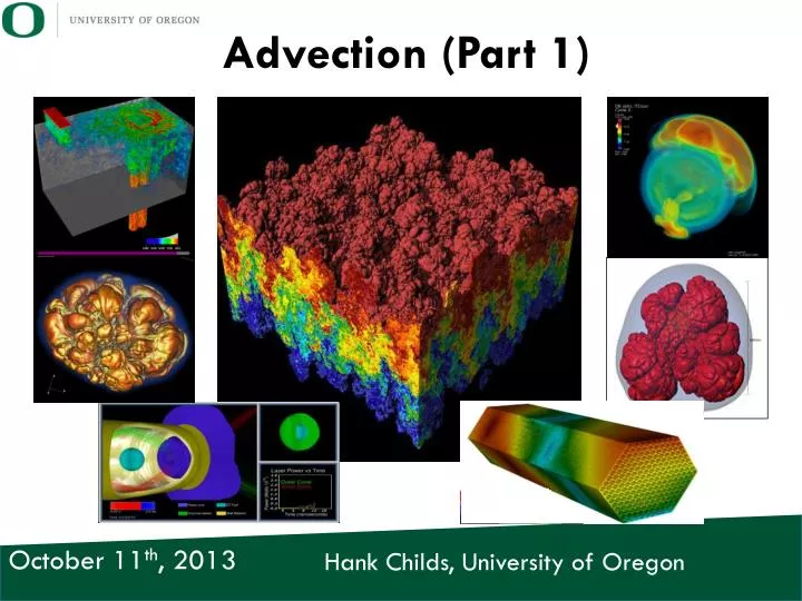
Advection (Part1) Hank Childs, University of Oregon October 11th,2013
Announcements • Bonus OH Mon 1-2 • Weds and Fri OH both canceled • Class canceled Weds • Makeup later in the quarter • Project 3 due Weds • Class on Fri the 18th will be held • Floating lecture on interpolation, fields, and meshes still coming
Announcements (cont’d) • My lecture style: • Go fast through content • Review content following lecture • Will be covering advection • Will likely feel fast • Will review it on Fri the 18th
Project 3 • Assigned October 9th, prompt online • Due October 16th, midnight ( October 17th, 6am) • Worth 5% of your grade • Provide: • Code skeleton online • Correct answers provided • You send me: • source code • three images from your program
Project 3 in a nutshell • I give you a 2D data set. • You will produce 3 images that are 500x500 pixels. • The 2D data set will be mapped on to the pixels. • Pixel (0,0): X=-9, Y=-9 • Pixel (499, 0): X=+9, Y=-9, pixel (0,499): X=-9, Y=+9 • Pixel (499,499): X=+9, Y=+9
Project 3 in a nutshell • For each of the 250,000 pixels (500x500), you will apply 3 color maps to a scalar field
Particle advection is the foundation to many visualization algorithms Advection will require us to evaluate velocity at arbitrary locations.
LERPing vectors X = B-A A B } t X A A+t*X • LERP = Linear Interpolate • Goal: interpolate vector between A and B. • Consider vector X, where X = B-A • A + t*(B-A) = A+t*X • Takeaway: • you can LERP the components individually • the above provides motivation for why this works
Quiz Time: LERPing vectors F(11,13) = (6,1) F(10,13) = (1,1) What is value of F(10.3, 12)? Answer: (-0.4, 2.9) F(10,12) = (-1, 2) F(11,12) = (1,5)
Particle advection is the foundation to many visualization algorithms Courtesy C. Garth, Kaiserslautern
Overview of advection process • Place a massless particle at a seed location • Displace the particle according to the vector field • Result is an “integral curve” corresponding to the trajectory the particle travels • Math gets tricky What would be the difference between a massless and “mass-ful” particle?
Formal definition for particle advection • Output is an integral curve, S, which follows trajectory of the advection • S(t) = position of curve at time t • S(t0) = p0 • t0: initial time • p0: initial position • S’(t) = v(t, S(t)) • v(t, p): velocity at time t and position p • S’(t): derivative of the integral curve at time t This is an ordinary differential equation (ODE).
The integral curve for particle advection is calculated iteratively S(t0) = p0 while (ShouldContinue()) { S(ti) = AdvanceStep(S(t(i-1)) } Many possible criteria for ShouldContinue. For now, assume fixed number of steps.
Integral curve calculation with a fixed number of steps S0 = P0 for (inti = 1 ; i < numSteps ; i++) { Si = AdvanceStep(S(i-1)) } How to do an advance?
AdvanceStep goal: to calculate Si from S(i-1) S0 S1 = AdvanceStep(S0) S4 = AdvanceStep(S3) S5= AdvanceStep(S4) S2 = AdvanceStep(S1) S3= AdvanceStep(S2) S1 S3 S4 S2 S5 This picture is misleading: steps are typically much smaller.
AdvanceStep Overview • Think of AdvanceStep as a function: • Input arguments: • S(i-1): Position, time • Output arguments: • Si: New position, new time (later than input time) • Optional input arguments: • More parameters to control the stepping process.
AdvanceStep Overview • Different numerical methods for implementing AdvanceStep: • Simplest version: Euler step • Most common: Runge-Kutta-4 (RK4) • Several others as well
Euler Method • Most basic method for solving an ODE • Idea: • First, choose step size: h. • Second,AdvanceStep(pi, ti) returns: • New position: pi+1 = pi+h*v(ti, pi) • New time: ti+1 = ti+h
Quiz Time: Euler Method • Euler Method: • New position: pi+1 = pi+h*v(ti, pi) • New time: ti+1 = ti+h • Let h=0.01s • Let p0 = (1,2,1) • Let t0 = 0s • Let v(p0, t0) = (-1, -2, -1) • What is (p1, t1) if you are using an Euler method? Answer: ((0.99, 1.98, 0.99), 0.01)
Quiz Time #2: Euler Method • Euler Method: • New position: pi+1 = pi+h*v(ti, pi) • New time: ti+1 = ti+h • Let h=0.01s • Let p1 = (0.99,1.98,0.99) • Let t1 = 0.01s • Let v(p1, t1) = (1, 2, 1) • What is (p2, t2) if you are using an Euler method? Answer: ((1, 2, 1), 0.02)
Quiz Time #3: Euler Method • Euler Method: • New position: pi+1 = pi+h*v(ti, pi) • New time: ti+1 = ti+h • Let h=0.01s • Let p2 = (1,2,1) • Let t2 = 0.02s • Let v(p2, t2) = (1, 0, 0) • What is (p3, t3) if you are using an Euler method? Answer: ((1.01, 2, 1), 0.03)
Euler Method: Pros and Cons • Pros: • Simple to implement • Computationally very efficient • (quiz) Cons: • Prone to inaccuracy • Above statements are an oversimplification: • Can be very accurate with small steps size, but then also very inefficient. • Can be very fast, but then also inaccurate.
Quiz Time • You want to perform a particle advection. • What inputs do you need? • Velocity field • Step size • Termination criteria / # of steps • Initial seed position / time
Quiz Time • Write down pseudo-code to do advection with an Euler step: • Initial seed location: (0,0,0) • Initial seed time: 0s • Step size = 0.01s • Velocity field: v • Termination criteria: advance 0.1s (take 10 steps) • Function to evaluate velocity: • EvaluateVelocity(position, time)
Quiz Time (answer) S[0] = (0,0,0); time = 0; for (inti = 0 ; i < 10 ; i++) { S[i+1] = S[i]+h*EvaluateVelocity(S[i], time); time += h; }
Runge-Kutta Method (RK4) • Most common method for solving an ODE • Definition: • First, choose step size, h. • Second,AdvanceStep(pi, ti) returns: • New position: pi+1 = pi+(1/6)*h*(k1+2k2+2k3+k4) • k1 = v(ti, pi) • k2 = v(ti + h/2, pi + h/2*k1) • k3= v(ti + h/2, pi + h/2*k2) • k4= v(ti + h, pi + h*k3) • New time: ti+1 = ti+h
Physical interpretation of RK4 • New position: pi+1 = pi+(1/6)*h*(k1+2k2+2k3+k4) • k1 = v(ti, pi) • k2 = v(ti + h/2, pi + h/2*k1) • k3= v(ti + h/2, pi + h/2*k2) • k4= v(ti + h, pi + h*k3) v(ti+h, pi+h*k3) = k4 pi pi+ h/2*k2 pi+ h*k3 v(ti+h/2, pi+h/2*k2) = k3 v(ti, pi) = k1 pi+ h/2*k1 v(ti+h/2, pi+h/2*k1) = k2 Evaluate 4 velocities, use combination to calculate pi+1
Quiz time: Runge-Kutta 4 • Just kidding
Runge-Kuttavs Euler • Euler Method: • “1st order numerical method for solving ordinary differential equations (ODEs)” error per step is O(h2), total error is O(h) • Runge-Kutta: • “4th order numerical method for solving ODEs” error per step is O(h5), total error is O(h4) • Intuition: all of RK4’s “look-aheads” prevents you from stepping too far into the wrong place. h is small, so hx is smaller still
Quiz Time: RK4 vs Euler • Let h=0.01s • How many velocity field evaluations for RK4 to advance 1s? • How many velocity field evaluations for Euler to advance 1s? 400 for RK4, 100 for Euler
Quiz Time: RK4 vs Euler • Let h=0.01 for an RK4 • What h for Euler to achieve similar accuracy? • Error for RK4 is: O(1e-2^4) = O(1e-8) • Error for Euler is: O(h^2) --- > h=1e-4 • What is the ratio of velocity evaluations for Euler to achieve same accuracy? 25X more for Euler
Other ODE solvers • Adams/Bashforth, Dormand/Prince are also used • Idea: adaptive step size. • If the field is homogeneous, then take a bigger step size (bigger h) • If the field is heterogeneous, then take a smaller step size • Quiz: why would you want to do this? Answer: great accuracy at reduced computational cost
Termination criteria • Time
Termination criteria • Time • Distance
Termination criteria • Time • Distance • Number of steps • Same as time? • Other advanced criteria, based on particle advection purpose
Other reasons for advection termination • Exit the volume
Other reasons for advection termination • Advect into a sink
Steady versus Unsteady State • Unsteady state: the velocity field evolves over time • Steady state: the velocity field has reached steady state and remains unchanged as time evolves
Most common particle advection technique: streamlines and pathlines • Idea: plot the entire trajectory of the particle all at one time. Streamlines in the “fish tank”
Streamline vsPathlines • Streamlines: plot trajectory of a particle from a steady state field • Pathlines: plot trajectory of a particle from an unsteady state field • Quiz: most common configuration? • Neither!! • Pretend an unsteady state field is actually steady state and plot streamlines from one moment in time. • Quiz: why would anyone want to do this? • (answer: performance)
Lots more to talk about • How do we pragmatically deal with unsteady state flow (velocities that change over time)? • More operations based on particle advection • Stability of results
Project 4 • Will be available next week • There will be OH time before it is due • Still lining up data • You will be asked to: • perform RK4 integration • interpolate the vector field • generate streamline output