Download
1 / 19
190 likes | 328 Views
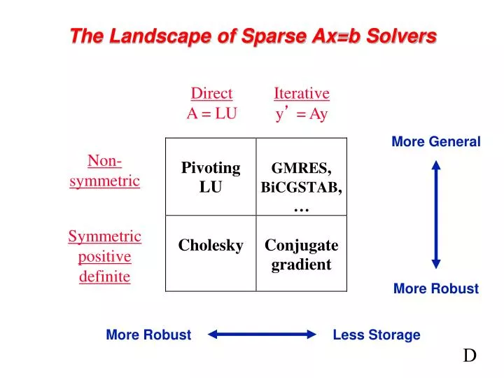
Direct A = LU. Iterative y ’ = Ay. More General. Non- symmetric. Symmetric positive definite. More Robust. More Robust. Less Storage. The Landscape of Sparse Ax=b Solvers. D. Four views of the conjugate gradient method. To solve Ax = b, where A is symmetric and positive definite.

E N D
Direct A = LU Iterative y’ = Ay More General Non- symmetric Symmetric positive definite More Robust More Robust Less Storage The Landscape of Sparse Ax=b Solvers D
Four views of the conjugate gradient method To solve Ax = b, where A is symmetric and positive definite. • Operational view • Orthogonal sequences view • Optimization view • Convergence view
Four views of the conjugate gradient method To solve Ax = b, where A is symmetric and positive definite. • Operational view • Orthogonal sequences view • Optimization view • Convergence view
Conjugate gradient iteration for Ax = b x0 = 0 approx solution r0 = b residual = b - Ax d0 = r0 search direction for k = 1, 2, 3, . . . xk = xk-1 + … new approx solution rk = … new residual dk = … new search direction
Conjugate gradient iteration for Ax = b x0 = 0 approx solution r0 = b residual = b - Ax d0 = r0 search direction for k = 1, 2, 3, . . . αk = … step length xk = xk-1 + αk dk-1 new approx solution rk = … new residual dk = … new search direction
Conjugate gradient iteration for Ax = b x0 = 0 approx solution r0 = b residual = b - Ax d0 = r0 search direction for k = 1, 2, 3, . . . αk = (rTk-1rk-1) / (dTk-1Adk-1) step length xk = xk-1 + αk dk-1 new approx solution rk = … new residual dk = … new search direction
Conjugate gradient iteration for Ax = b x0 = 0 approx solution r0 = b residual = b - Ax d0 = r0 search direction for k = 1, 2, 3, . . . αk = (rTk-1rk-1) / (dTk-1Adk-1) step length xk = xk-1 + αk dk-1 new approx solution rk = … new residual βk = (rTk rk) / (rTk-1rk-1) dk = rk + βk dk-1 new search direction
Conjugate gradient iteration for Ax = b x0 = 0 approx solution r0 = b residual = b - Ax d0 = r0 search direction for k = 1, 2, 3, . . . αk = (rTk-1rk-1) / (dTk-1Adk-1) step length xk = xk-1 + αk dk-1 new approx solution rk = rk-1 – αk Adk-1 new residual βk = (rTk rk) / (rTk-1rk-1) dk = rk + βk dk-1 new search direction
Conjugate gradient iteration x0 = 0, r0 = b, d0 = r0 for k = 1, 2, 3, . . . αk = (rTk-1rk-1) / (dTk-1Adk-1) step length xk = xk-1 + αk dk-1 approx solution rk = rk-1 – αk Adk-1 residual βk = (rTk rk) / (rTk-1rk-1) improvement dk = rk + βk dk-1 search direction • One matrix-vector multiplication per iteration • Two vector dot products per iteration • Four n-vectors of working storage
Four views of the conjugate gradient method To solve Ax = b, where A is symmetric and positive definite. • Operational view • Orthogonal sequences view • Optimization view • Convergence view
Krylov subspaces • Eigenvalues: Av = λv { λ1, λ2 , . . ., λn} • Cayley-Hamilton theorem implies (A – λ1I)·(A – λ2I) · · · (A – λnI) = 0 ThereforeΣ ciAi = 0 for someci so A-1 = Σ (–ci/c0)Ai–1 • Krylov subspace: Therefore if Ax = b, then x = A-1 b and x span (b, Ab, A2b, . . ., An-1b) = Kn (A, b) 0 i n 1 i n
Conjugate gradient: Orthogonal sequences • Krylov subspace: Ki (A, b)= span (b, Ab, A2b, . . ., Ai-1b) • Conjugate gradient algorithm:for i = 1, 2, 3, . . . find xi Ki (A, b) such that ri= (b – Axi) Ki (A, b) • Notice ri Ki+1 (A, b), sorirj for all j < i • Similarly, the “directions” are A-orthogonal:(xi – xi-1 )T·A·(xj – xj-1 ) = 0 • The magic: Short recurrences. . .A is symmetric => can get next residual and direction from the previous one, without saving them all.
Four views of the conjugate gradient method To solve Ax = b, where A is symmetric and positive definite. • Operational view • Orthogonal sequences view • Optimization view • Convergence view
Four views of the conjugate gradient method To solve Ax = b, where A is symmetric and positive definite. • Operational view • Orthogonal sequences view • Optimization view • Convergence view
Conjugate gradient: Convergence • In exact arithmetic, CG converges in n steps (completely unrealistic!!) • Accuracy after k steps of CG is related to: • consider polynomials of degree k that are equal to 1 at 0. • how small can such a polynomial be at all the eigenvalues of A? • Thus, eigenvalues close together are good. • Condition number:κ(A) = ||A||2 ||A-1||2 = λmax(A) / λmin(A) • Residual is reduced by a constant factor by O(κ1/2(A)) iterations of CG.
n1/2 n1/3 Complexity of direct methods Time and space to solve any problem on any well-shaped finite element mesh
n1/2 n1/3 Complexity of linear solvers Time to solve model problem (Poisson’s equation) on regular mesh
Hierarchy of matrix classes (all real) • General nonsymmetric • Diagonalizable • Normal • Symmetric indefinite • Symmetric positive (semi)definite = Factor width n • Factor width k . . . • Factor width 4 • Factor width 3 • Diagonally dominant SPSD = Factor width 2 • Generalized Laplacian = Symm diag dominant M-matrix • Graph Laplacian
Other Krylov subspace methods • Nonsymmetric linear systems: • GMRES: for i = 1, 2, 3, . . . find xi Ki (A, b) such that ri= (Axi – b) Ki (A, b)But, no short recurrence => save old vectors => lots more space (Usually “restarted” every k iterations to use less space.) • BiCGStab, QMR, etc.:Two spaces Ki (A, b)and Ki (AT, b)w/ mutually orthogonal basesShort recurrences => O(n) space, but less robust • Convergence and preconditioning more delicate than CG • Active area of current research • Eigenvalues: Lanczos (symmetric), Arnoldi (nonsymmetric)