APPLICATION OF PARTIAL DIFFERENTIATION

1. APPLICATION OF PARTIAL DIFFERENTIATION RITU DAVE DEPARTMENT OF MATHEMATICS

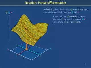
2. Tangent Planes and LinearApproximations • Suppose a surface S has equation z = f (x,y),where f has continuous first partial derivatives, and let P(x0, y0, z0) be a pointon S. Let C1 and C2 be the two curves obtained by intersection the vertical planes y = y0 and x = x0 with the surface. Thus, point P lies on both C1andC2. Let T1 and T2 be the tangentlines to the curvesC1andC2at point P. Then thetangent planeto the surface S at point P is defined to be the plane that contains both tangent lines T1 andT2.

3. Tangent Planes and LinearApproximations • Suppose a surface S has equation z = f(x, y), wheref • has continuous first partialderivatives. • Let P(x0, y0, z0) be a point onS. • We know from Equation that any plane passing through thepoint • P(x0, y0,z0)has an equation of theform • zz0 fx(x0,y0)(xx0)fy(x0,y0)(yy0)

4. LINEAR APPROXIMATIONAND LINEARIZATION • Thelinearizationof f at (a, b) is the linear functions whose graph is the tangent plane,namely • L(x,y)f (a,b)fx(a,b)(xa)fy(a,b)(yb) • The approximation • f (x,y)f (a,b)fx(a,b)(xa)fy(a,b)(yb) • is called thelinear approximationortangent planeapproximationof f at (a,b).

5. LINEAR APPROXIMATIONAND LINEARIZATION • Recall that Δx and Δy areincrementsof x and y, respectively. If z = f(x,y) is a function of two variables, then Δz, theincrementof z is defined tobe • Δz = f (x + Δx, y + Δy) − f (x,y) • If z = f (x,y),then f isdifferentiableat (a, b) if Δz can be expressed in theform • where ε1 and ε2→0 as (Δx, Δy) → (0,0).

6. LINEAR APPROXIMATIONAND LINEARIZATION • Theorem: If thepartial derivatives fx and fy exist • near (a, b)and are continuousat(a, b), then f is differentiable at (a,b). • For a differentiable function of two variables, z = f (x, y), we define thedifferentialsdx and dy to be independentvariables. Then thedifferentialdz, also called thetotal differential, is defined by dzf (a,b)dxf (a,b)dyzdxzdy x y xy

7. LINEAR APPROXIMATIONAND LINEARIZATION • For a function of three variables, w = f (x, y,z): • 1. Thelinear approximationat (a, b, c)is • f(x,y,z)f(a,b,c)fx(a,b,c)(xa)fy(a,b,c)(yb)fz(a,b,c)(zc) • 2. Theincrementof wis • wf (xx, yy,zz)f(x,y,z) • 3. Thedifferentialdw is • dwwdxwdywdz • x y z

8. TAYLOR’sEXPANSIONS • Letafunction fxbe given as the sum of a power series in the convergence interval of the powerseries •  n f xa xx n 0 n0 • Then such a power series is unique andits coefficients are given by theformula   n f x 0 a  n  n!

9. TAYLOR’sEXPANSIONS • If afunction fxhas derivatives of all orders at x0, then we can formally write the corresponding Taylor series f 'x0f ''x0f '''x0  f xf x0  xx0xx0xx0 2 3 1!2!3! • The power series created in this way is then called the Taylor series ofthefunction f x. A Taylor seriesfor x0 0 is called MacLaurinseries.

10. TAYLOR’sEXPANSIONS • Therearefunctions f(x) • whose formally generated Taylor series do not converge toit. • A condition that guarantees that this will not happen saysthat • the derivatives of f (x) are all uniformlybounded • in a neighbourhood ofx0.

11. TAYLOR’sEXPANSIONS • There are functions with aTaylorseries that, as a power series, converges to quite a different function as the following exampleshows: 1 f xe f 00 x2 Example for x 0,

12. TAYLOR’sEXPANSIONS x 0 1  x2 de  1 2 2  dx f 'x x2  e  x3 1 x3ex2 and for x =0: 1 x 1 x2 e 0 1 t 1 f 'xlim lim lim lim lim 0 t et t 2tet 1 1 2 2 x x0 x0 x0 ex xex 2 2

13. TAYLOR’sEXPANSIONS In a similar way, we could also showthat 0 f 0f '0f ' 0f k 0 This means that the Taylor series corresponding to f (x) converges toa constant function that is equal to zero at all points. Butclearly, for any . 1 x2 x 0 e 0

14. TAYLOR’sEXPANSIONS Taylor series of somefunctions: x2 x3 x x e 1  1!2!3! x3 x5 x7 sin x x  3!5!7! x2 x4 x6 cosx1  2!4!6! x2 x3 x4 ln1xx  2 3 4

15. Maxima andMinima • The Least and theGreatest • Many problems that arise in mathematics call for finding the largest and smallest values that a differentiable function can assume on a particular domain. • There is a strategy for solving these applied problems.

16. Maxima andMinima • The Max-Min Theorem for ContinuousFunctions • If f is a continuous function at every point of a closed interval[a.b],then f takes on aminimum value, m, and a maximum value, M, on[a,b]. • In other words, a function that is continuous on a closed interval takes on a maximum and a minimum on thatinterval.

17. Maxima andMinima • The Max-Min Theorem,Graphically

18. Maxima andMinima • Strategy for Max-MinProblems • The main problem is setting up theequation: • Drawapicture. Label the parts that are important for the problem. Keep track of what the variablesrepresent. • Use a known formula for the quantity to be maximizedor minimized. • Writeanequation. Try to express the quantity that is to be maximized or minimized as a function of a single variable, sayy=f(x). This may require some algebraand the use of information from theproblem.

19. Maxima andMinima • Find an interval of values forthisvariable. Youneed to be mindful of the domain based on restrictions in theproblem. • Test the critical points andthe endpoints. The extreme valueof f will be found among the values f takes at the endpoints of the domain and at the points where the derivative is zero or fails toexist. • List the values of f atthesepoints. If f has an absolute maximum or minimum on its domain, it will appear on thelist. You may have to examine the sign pattern of the derivative or the sign of the second derivative to decide whether a given value represents a max, min orneither.

20. LAGRANGE METHOD • Many times a stationary value of the function of several variables which are not all independent but connected by some relationship is needed to be known. Generally, we do convert the given functions to the one, having least number of independent variables with the help of these relations, then it solved. But this not always be necessary to solve such functions using this ordinary method, and when this procedure become impractical, Lagrange’s method proves to be very convenient, which is explained in the ongoing lines.

21. LAGRANGE METHOD • Let be a function ofthree variables whichare connected by the relation • For u to be have stationary value, it is necessarythat • Also the differential of the relationshipfunction

22. LAGRANGE METHOD • Multiply (2) by parameter λ and add to (1). Then we obtain theexpression • To satisfy this equation the components of the expression need to be equal to zero,i.e. • This three equations together with the relationship functioni.e. will determine thevalueof and λ for which u isstationary.

23. THANK YOU