Learning for Text Categorization: Algorithms and Methods

1. Text Categorization

2. Categorization • Given: • A description of an instance, xX, where X is the instance language or instance space. • A fixed set of categories: C={c1, c2,…cn} • Determine: • The category of x: c(x)C, where c(x) is a categorization function whose domain is X and whose range is C.

3. Learning for Categorization • A training example is an instance xX, paired with its correct category c(x): <x, c(x)> for an unknown categorization function, c. • Given a set of training examples, D. • Find a hypothesized categorization function, h(x), such that: Consistency

4. Sample Category Learning Problem • Instance language: <size, color, shape> • size  {small, medium, large} • color  {red, blue, green} • shape  {square, circle, triangle} • C = {positive, negative} • D:

5. General Learning Issues • Many hypotheses are usually consistent with the training data. • Bias • Any criteria other than consistency with the training data that is used to select a hypothesis. • Classification accuracy (% of instances classified correctly). • Measured on independent test data. • Training time (efficiency of training algorithm). • Testing time (efficiency of subsequent classification).

6. Generalization • Hypotheses must generalize to correctly classify instances not in the training data. • Simply memorizing training examples is a consistent hypothesis that does not generalize. • Occam’s razor: • Finding a simple hypothesis helps ensure generalization.

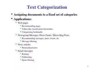
7. Text Categorization • Assigning documents to a fixed set of categories. • Applications: • Web pages • Recommending • Yahoo-like classification • Newsgroup Messages • Recommending • spam filtering • News articles • Personalized newspaper • Email messages • Routing • Prioritizing • Folderizing • spam filtering

8. Learning for Text Categorization • Manual development of text categorization functions is difficult. • Learning Algorithms: • Bayesian (naïve) • Neural network • Relevance Feedback (Rocchio) • Rule based (Ripper) • Nearest Neighbor (case based) • Support Vector Machines (SVM)

9. Using Relevance Feedback (Rocchio) • Relevance feedback methods can be adapted for text categorization. • Use standard TF/IDF weighted vectors to represent text documents (normalized by maximum term frequency). • For each category, compute a prototype vector by summing the vectors of the training documents in the category. • Assign test documents to the category with the closest prototype vector based on cosine similarity.

10. Rocchio Text Categorization Algorithm(Training) Assume the set of categories is {c1, c2,…cn} For i from 1 to n let pi = <0, 0,…,0> (init. prototype vectors) For each training example <x, c(x)> D Let d be the frequency normalized TF/IDF term vector for doc x Let i = j: (cj = c(x)) (sum all the document vectors in ci to get pi) Let pi = pi + d

11. Rocchio Text Categorization Algorithm(Test) Given test document x Let d be the TF/IDF weighted term vector for x Let m = –2 (init.maximum cosSim) For i from 1 to n: (compute similarity to prototype vector) Let s = cosSim(d, pi) if s > m let m = s let r = ci (update most similar class prototype) Return class r

12. Illustration of Rocchio Text Categorization

13. Rocchio Properties • Does not guarantee a consistent hypothesis. • Forms a simple generalization of the examples in each class (a prototype). • Prototype vector does not need to be averaged or otherwise normalized for length since cosine similarity is insensitive to vector length. • Classification is based on similarity to class prototypes.

14. Rocchio Time Complexity • Note: The time to add two sparse vectors is proportional to minimum number of non-zero entries in the two vectors. • Training Time: O(|D|(Ld + |Vd|)) = O(|D| Ld) where Ld is the average length of a document in D and Vd is the average vocabulary size for a document in D. • Test Time: O(Lt + |C||Vt|) where Lt is the average length of a test document and |Vt | is the average vocabulary size for a test document. • Assumes lengths of pi vectors are computed and stored during training, allowing cosSim(d, pi) to be computed in time proportional to the number of non-zero entries in d (i.e. |Vt|)

15. Nearest-Neighbor Learning Algorithm • Learning is just storing the representations of the training examples in D. • Testing instance x: • Compute similarity between x and all examples in D. • Assign x the category of the most similar example in D. • Does not explicitly compute a generalization or category prototypes. • Also called: • Case-based • Memory-based • Lazy learning

16. K Nearest-Neighbor • Using only the closest example to determine categorization is subject to errors due to: • A single atypical example. • Noise (i.e. error) in the category label of a single training example. • More robust alternative is to find the k most-similar examples and return the majority category of these k examples. • Value of k is typically odd to avoid ties, 3 and 5 are most common.

17. Similarity Metrics • Nearest neighbor method depends on a similarity (or distance) metric. • Simplest for continuous m-dimensional instance space is Euclidian distance. • Simplest for m-dimensional binary instance space is Hamming distance (number of feature values that differ). • For text, cosine similarity of TF-IDF weighted vectors is typically most effective.

18. 3 Nearest Neighbor Illustration(Euclidian Distance) . . . . . . . . . . .

19. K Nearest Neighbor for Text Training: For each eachtraining example <x, c(x)> D Compute the corresponding TF-IDF vector, dx, for document x Test instance y: Compute TF-IDF vector d for document y For each <x, c(x)> D Let sx = cosSim(d, dx) Sort examples, x, in D by decreasing value of sx Let N be the first k examples in D. (get most similar neighbors) Return the majority class of examples in N

20. Illustration of 3 Nearest Neighbor for Text

21. Rocchio Anomoly • Prototype models have problems with polymorphic (disjunctive) categories.

22. 3 Nearest Neighbor Comparison • Nearest Neighbor tends to handle polymorphic categories better.

23. Nearest Neighbor Time Complexity • Training Time: O(|D| Ld) to compose TF-IDF vectors. • Testing Time: O(Lt + |D||Vt|) to compare to all training vectors. • Assumes lengths of dxvectors are computed and stored during training, allowing cosSim(d, dx) to be computed in time proportional to the number of non-zero entries in d (i.e. |Vt|) • Testing time can be high for large training sets.

24. Nearest Neighbor with Inverted Index • Determining k nearest neighbors is the same as determining the k best retrievals using the test document as a query to a database of training documents. • Testing Time: O(B|Vt|) where B is the average number of training documents in which a test-document word appears. • Therefore, overall classification is O(Lt + B|Vt|) • Typically B << |D|

25. Bayesian Methods • Learning and classification methods based on probability theory. • Bayes theorem plays a critical role in probabilistic learning and classification. • Uses prior probability of each category given no information about an item. • Categorization produces a posterior probability distribution over the possible categories given a description of an item.

26. Axioms of Probability Theory • All probabilities between 0 and 1 • True proposition has probability 1, false has probability 0. P(true) = 1 P(false) = 0. • The probability of disjunction is: B A

27. Conditional Probability • P(A | B) is the probability of A given B • Assumes that B is all and only information known. • Defined by: B A

28. Independence • A and B are independent iff: • Therefore, if A and B are independent: These two constraints are logically equivalent

29. Bayes Theorem Simple proof from definition of conditional probability: (Def. cond. prob.) (Def. cond. prob.) QED:

30. Bayesian Categorization • Letset of categories be {c1, c2,…cn} • Let E be description of an instance. • Determine category of E by determining for each ci • P(E) can be determined since categories are complete and disjoint.

31. Bayesian Categorization (cont.) • Need to know: • Priors: P(ci) • Conditionals: P(E | ci) • P(ci) are easily estimated from data. • If ni of the examples in D are in ci,then P(ci) = ni / |D| • Assume instance is a conjunction of binary features: • Too many possible instances (exponential in m) to estimate all P(E | ci)

32. Naïve Bayesian Categorization • If we assume features of an instance are independent given the category (ci) (conditionally independent). • Therefore, we then only need to know P(ej | ci) for each feature and category.

33. Naïve Bayes Example • C = {allergy, cold, well} • e1 = sneeze; e2 = cough; e3 = fever • E = {sneeze, cough, fever}

34. Naïve Bayes Example (cont.) P(well | E) = (0.9)(0.1)(0.1)(0.99)/P(E)=0.0089/P(E) P(cold | E) = (0.05)(0.9)(0.8)(0.3)/P(E)=0.01/P(E) P(allergy | E) = (0.05)(0.9)(0.7)(0.6)/P(E)=0.019/P(E) Most probable category: allergy P(E) = 0.089 + 0.01 + 0.019 = 0.0379 P(well | E) = 0.23 P(cold | E) = 0.26 P(allergy | E) = 0.50 E={sneeze, cough, fever}

35. Estimating Probabilities • Normally, probabilities are estimated based on observed frequencies in the training data. • If D contains niexamples in category ci, and nij of these ni examples contains feature ej, then: • However, estimating such probabilities from small training sets is error-prone. • If due only to chance, a rare feature, ek, is always false in the training data, ci :P(ek | ci) = 0. • If ek then occurs in a test example, E, the result is that ci: P(E | ci) = 0 and ci: P(ci | E) = 0

36. Smoothing • To account for estimation from small samples, probability estimates are adjusted or smoothed. • Laplace smoothing using an m-estimate assumes that each feature is given a prior probability, p, that is assumed to have been previously observed in a “virtual” sample of size m. • For binary features, p is simply assumed to be 0.5.

37. Naïve Bayes for Text • Modeled as generating a bag of words for a document in a given category by repeatedly sampling with replacement from a vocabulary V = {w1, w2,…wm} based on the probabilities P(wj| ci). • Smooth probability estimates with Laplace m-estimates assuming a uniform distribution over all words (p = 1/|V|) and m = |V| • Equivalent to a virtual sample of seeing each word in each category exactly once.

38. Text Naïve Bayes Algorithm(Train) Let V be the vocabulary of all words in the documents in D For each category ci  C Let Dibe the subset of documents in D in category ci P(ci) = |Di| / |D| Let Ti be the concatenation of all the documents in Di Let ni be the total number of word occurrences in Ti For each word wj  V Let nij be the number of occurrences of wj in Ti Let P(wi| ci) = (nij + 1) / (ni + |V|)

39. Text Naïve Bayes Algorithm(Test) Given a test document X Let n be the number of word occurrences in X Return the category: where ai is the word occurring the ith position in X

40. Naïve Bayes Time Complexity • Training Time: O(|D|Ld + |C||V|)) where Ld is the average length of a document in D. • Assumes V and all Di , ni, and nij pre-computed in O(|D|Ld) time during one pass through all of the data. • Generally just O(|D|Ld) since usually |C||V| < |D|Ld • Test Time: O(|C| Lt) where Lt is the average length of a test document. • Very efficient overall, linearly proportional to the time needed to just read in all the data. • Similar to Rocchio time complexity.

41. Underflow Prevention • Multiplying lots of probabilities, which are between 0 and 1 by definition, can result in floating-point underflow. • Since log(xy) = log(x) + log(y), it is better to perform all computations by summing logs of probabilities rather than multiplying probabilities. • Class with highest final un-normalized log probability score is still the most probable.

42. Naïve Bayes Posterior Probabilities • Classification results of naïve Bayes (the class with maximum posterior probability) are usually fairly accurate. • However, due to the inadequacy of the conditional independence assumption, the actual posterior-probability numerical estimates are not. • Output probabilities are generally very close to 0 or 1.

43. Evaluating Categorization • Evaluation must be done on test data that are independent of the training data (usually a disjoint set of instances). • Classification accuracy: c/n where n is the total number of test instances and c is the number of test instances correctly classified by the system. • Results can vary based on sampling error due to different training and test sets. • Average results over multiple training and test sets (splits of the overall data) for the best results.

44. N-Fold Cross-Validation • Ideally, test and training sets are independent on each trial. • But this would require too much labeled data. • Partition data into N equal-sized disjoint segments. • Run N trials, each time using a different segment of the data for testing, and training on the remaining N1 segments. • This way, at least test-sets are independent. • Report average classification accuracy over the N trials. • Typically, N = 10.

45. Learning Curves • In practice, labeled data is usually rare and expensive. • Would like to know how performance varies with the number of training instances. • Learning curves plot classification accuracy on independent test data (Y axis) versus number of training examples (X axis).

46. N-Fold Learning Curves • Want learning curves averaged over multiple trials. • Use N-fold cross validation to generate N full training and test sets. • For each trial, train on increasing fractions of the training set, measuring accuracy on the test data for each point on the desired learning curve.

47. Sample Learning Curve(Yahoo Science Data)

48. References • Fabrizio Sebastiani. Machine Learning in Automated Text Categorization. ACM Computing Surveys, 34(1):1-47, 2002. • Tom Mitchell, Machine Learning. McGraw-Hill, 1997. • Yiming Yang & Xin Liu, A re-examination of text categorization methods. Proceedings of SIGIR, 1999. • Evaluating and Optimizing Autonomous Text Classification Systems (1995) David Lewis. Proceedings of the 18th Annual International ACM SIGIR Conference on Research and Development in Information Retrieval • Foundations of Statistical Natural Language Processing. Chapter 16. MIT Press. Manning and Schütze. • Trevor Hastie, Robert Tibshirani and Jerome Friedman, Elements of Statistical Learning: Data Mining, Inference and Prediction. Springer-Verlag, New York.