Experiment Design Overview

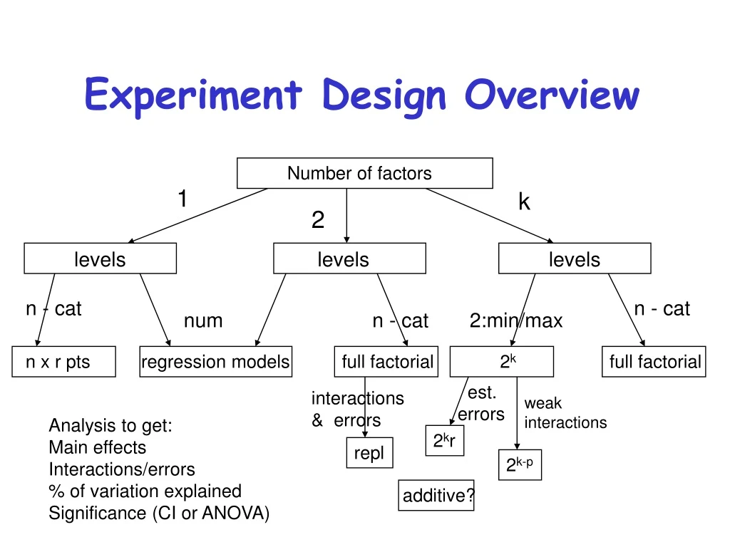
1. additive? Experiment Design Overview Number of factors 1 k 2 levels levels levels n - cat n - cat num n - cat 2:min/max n x r pts regression models full factorial 2k full factorial est.errors interactions& errors weakinteractions Analysis to get: Main effects Interactions/errors % of variation explained Significance (CI or ANOVA) 2kr repl 2k-p

2. Two-Factor Full Factorial Design Without Replications • Used when you have only two parameters • But multiple levels for each • Test all combinations of the levels of the two parameters • At this point, without replicating any observations • For factors A and B with a and b levels, ab experiments required

3. Experimental Design (l1,0, l1,1, … , l1,n1-1) x (l2,0, l2,1, … , l2,n2-1) 2 different factors, each factor with nilevels (and possibly r replications -- defer) Categorical levels Factor 1 Factor 2

4. What is This Design Good For? • Systems that have two important factors • Factors are categorical • More than two levels for at least one factor • Examples - • Performance of different processors under different workloads • Characteristics of different compilers for different benchmarks • Effects of different reconciliation topologies and workloads on a replicated file system

5. What Isn’t This Design Good For? • Systems with more than two important factors • Use general factorial design • Non-categorical variables • Use regression • Only two levels • Use 22 designs

6. Model For This Design • yij is the observation • m is the mean response • j is the effect of factor A at level j • i is the effect of factor B at level i • eij is an error term • Sums of j’s and j’s are both zero

7. What Are the Model’s Assumptions? • Factors are additive • Errors are additive • Typical assumptions about errors • Distributed independently of factor levels • Normally distributed • Remember to check these assumptions!

8. Computing the Effects • Need to figure out , j, and j • Arrange observations in two-dimensional matrix • With b rows and a columns • Compute effects such that error has zero mean • Sum of error terms across all rows and columns is zero

9. Two-Factor Full Factorial Example • We want to expand the functionality of a file system to allow automatic compression • We examine three choices - • Library substitution of file system calls • A new VFS • UCLA stackable layers • Using three different benchmarks • With response time as the metric

10. Sample Data for Our Example Library VFS Layers Compile Benchmark 94.3 89.5 96.2 Email Benchmark 224.9 231.8 247.2 Web Server Benchmark 733.5 702.1 797.4

11. Computing  • Averaging the jth column, • By assumption, the error terms add to zero • Also, the js add to zero, so • Averaging rows produces • Averaging everything produces

12. So the Parameters Are . . .

13. Sample Data for Our Example Library VFS Layers Compile Benchmark 94.3 89.5 96.2 93.3 Email Benchmark 224.9 231.8 247.2 234.6 Web Server Benchmark 733.5 702.1 797.4 744.3 _____________________________________________________ 350.9 341.1 380.3 357.4

14. Calculating Parameters for Our Example •  = grand mean = 357.4 • j = (-6.5, -16.3, 22.8) • i = (-264.1, -122.8, 386.9) • So, for example, the model predicts that the email benchmark using a special-purpose VFS will take 357.4 - 16.3 -122.8 seconds • Which is 218.3 seconds

15. Estimating Experimental Errors • Similar to estimation of errors in previous designs • Take the difference between the model’s predictions and the observations • Calculate a Sum of Squared Errors • Then allocate the variation

16. Allocating Variation • Using the same kind of procedure we’ve used on other models, • SSY = SS0 + SSA + SSB + SSE • SST = SSY - SS0 • We can then divide the total variation between SSA, SSB, and SSE

17. Calculating SS0, SSA, and SSB • a and b are the number of levels for the factors

18. Allocation of Variation For Our Example • SSE = 2512 • SSY = 1,858,390 • SS0 = 1,149,827 • SSA = 2489 • SSB = 703,561 • SST=708,562 • Percent variation due to A - .35% • Percent variation due to B - 99.3% • Percent variation due to errors - .35%

19. Analysis of Variation • Again, similar to previous models • With slight modifications • As before, use an ANOVA procedure • With an extra row for the second factor • And changes in degrees of freedom • But the end steps are the same • Compare F-computed to F-table • Compare for each factor

20. Analysis of Variation for Our Example • MSE = SSE/[(a-1)(b-1)]=2512/[(2)(2)]=628 • MSA = SSA/(a-1) = 2489/2 = 1244 • MSB = SSB/(b-1) = 703,561/2 = 351,780 • F-computed for A = MSA/MSE = 1.98 • F-computed for B = MSB/MSE = 560 • The 95% F-table value for A & B = 6.94 • A is not significant, B is

21. Checking Our Results With Visual Tests • As always, check if the assumptions made by this analysis are correct • Using the residuals vs. predicted and quantile-quantile plots

22. Residuals Vs. Predicted Response for Example

23. What Does This Chart Tell Us? • Do we or don’t we see a trend in the errors? • Clearly they’re higher at the highest level of the predictors • But is that alone enough to call a trend? • Perhaps not, but we should take a close look at both the factors to see if there’s a reason to look further • And take results with a grain of salt

24. Quantile-Quantile Plot for Example

25. Confidence Intervals for Effects • Need to determine the standard deviation for the data as a whole • From which standard deviations for the effects can be derived • Using different degrees of freedom for each • Complete table in Jain, pg. 351

26. Standard Deviations for Our Example • se = 25 • Standard deviation of  - • Standard deviation of j - • Standard deviation of i -

27. Calculating Confidence Intervals for Our Example • Just the file system alternatives shown here • At 95% level, with 4 degrees of freedom • CI for library solution - (-39,26) • CI for VFS solution - (-49,16) • CI for layered solution - (-10,55) • So none of these solutions are 95% significantly different than the mean

28. Looking a Little Closer • Does this mean that none of the alternatives for adding the functionality are different? • Use contrasts to checkcontrasts – any linear combination of effects whose coeff add up to zero (ch. 18.5)

29. Looking a Little Closer • For example, is the library approach significantly better than layers? • Using contrast of library-layers, the confidence interval is (-58,-.5) (at 95%) • So library approach is better, with this confidence

30. Two-Factor Full Factorial Design With Replications • Replicating a full factorial design allows separating out the interactions between factors from experimental error • Without replicating implies assumption that interactions were negligible and could be viewed as errors. • Read Chapter 22

31. Full Factorial Design With k Factors (l1,0, l1,1, … , l1,n1-1) x (l2,0, l2,1, … , l2,n2-1) x … x (lk,0, lk,1, … , lk,nk-1) k different factors, each factor with nilevelsr replications • Informal techniques just to answer which combo is of levels is best – rank responses Factor 1 Factor 2 Factor k

32. !additive Experiment Design Overview Number of factors 1 k 2 levels levels levels n - cat n - cat num n - cat 2:min/max Jain ch 21 Jain ch 17 n x r pts regression models full factorial 2k full factorial Jain ch 20 est.errors Jain ch 23 interactions& errors Jain ch 14,15 weakinteractions 2kr Jain ch 19 Jain ch 22 repl Jain ch 18 2k-p log transform

33. For Discussion Project Proposal • Statement of hypothesis • Workload decisions • Metrics to be used • Method