The chi-squared statistic  2 N

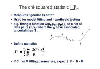
1. The chi-squared statistic 2N • Measures “goodness of fit” • Used for model fitting and hypothesis testing • e.g. fitting a function C(p1,p2,...pM; x) to a set of data pairs (xi,yi) where the yi have associated uncertainties i: • Define statistic: • If C has M fitting parameters, expect 2 ~ N - M

2. 2 fitting approach • Consider a set of data points Xi with a common mean <X> and individual errors i • We’ve already seen that the weighted average: • Alternatively use goodness of fit: • Find the value of A that minimises 

3. Parameter fitting by minimizing 2 • Set derivative of  w.r.t. A to zero and solve: • In other words, the optimally weighted average also minimizes .

4. 2 2min A Using 2 to estimate parameter uncertainties • Variance of optimally weighted average: • What is  for • Use Taylor series: • Now • So • Hence:

5. Error bars from 2 curvature • We’ve just seen that: • Hence 2≤1 encloses 68% of probability for A. • We use 2≤1 to get “1” error bars on the value of a single parameter fitted to data. • Use the second derivative (curvature): • For the case where • We get

6. Scaling a profile by 2 minimization • As before: • Xi = data, known. • i = error bars, known. • pi = profile, known. • A pi = profile scaled by factor A. • Goodness of fit:

7. Error bar on scale factor • Use the 2 curvature method. • Second derivative: • Use 2 = 1: 2 2min A