Download
1 / 11
140 likes | 359 Views
Chapter 3:Derivatives and Their Applications. By: Wishah Khalid, William Le, and Massuma. 3.1 – Higher-Order Derivatives, Velocity, and Acceleration(Part 1). The function y = f(x) has a first derivative y = f’(x). The second derivative of y = f(x) is the derivative of y = f’(x).

E N D
Chapter 3:Derivatives and Their Applications By: Wishah Khalid, William Le, and Massuma
3.1 – Higher-Order Derivatives, Velocity, and Acceleration(Part 1) • The function y = f(x) has a first derivative y = f’(x). The second derivative of y = f(x) is the derivative of y = f’(x). • To signify the second derivative, we put a second prime: f’’(x) or y’’. • The derivative of f(x) = 10x4 is f’(x) = 40x3. The second derivative is f’’(x) = 120x2. • For Leibniz’s notation, we put d2y/dx2. Example 1 Determine the second derivative of f(x) = x/1 + x when x = 1. Find the first derivative. f(x) = x(x + 1)-1 f’(x) = (1)(x + 1)-1 + (x)(-1)(x + 1)-2(1) f’(x) = (1/x + 1) – [x/(x + 1)2] f’(x) = [1(x + 1)/(x + 1)2] – [x/(x + 1)2] f’(x) = x + 1 – x/ (x + 1)2 f’(x) = 1/(x + 1)2 Find the second derivative. f’’(x) = -2(x + 1)-3(1) f’’(x) = -2/(x + 1)3 Now evaluate. f’’(1) = -2/(1 + 1)3 f’’(1) = -2/8 = -1/4
3.1 – Higher-Order Derivatives, Velocity, and Acceleration (Part 2) Velocity and Acceleration • The position of an object on a line relative to the origin is a function of time and commonly denoted by s(t). • The RoC of s(t) with respect to t is it’s velocity, v(t), and the RoC of velocity with respect to t is its acceleration, a(t). • In other words, v(t) = s’(t) and a(t) = v’(t) = s’’(t). • When v(t) > 0 and a(t) > 0, or v(t) < 0 and a(t) < 0, the object is accelerating. • Happens when the product of v(t) and a(t) are positive. • When v(t) > 0 and a(t) < 0, or v(t) < 0 and a(t) > 0, the object is decelerating. • Happens when the product of v(t) and a(t) are negative.
3.2 – Maximum and Minimum on an Interval (Extreme Values) Algorithm for Finding Maximum or Minimum (Extreme) Values If a function f(x) has a derivative at every point in the interval a ≤ x ≤ b, calculate f(x) at • all points in the interval a ≤ x ≤ b, where f’(x) = 0 • the endpoints x = a and x = b The maximum value of f(x) on the interval a ≤ x ≤ b is the largest of these values, and the minimum value of f(x) on the interval is the smallest of these values. Example 1 Find the extreme values of the function f(x) = -2x3 + 9x2 + 4 on the interval x ԑ [-1, 5]. f’(x) = -6x2 + 18x 0 = -6x(x – 3), f’(x) = 0 when x = 0 or x = 3. f(-1) = 15 f(0) = 4 f(3) = 31 -> Maximum f(5) = -21 -> Minimum Therefore, the maximum value of f(x) on the interval -1 ≤ x ≤ 5 is f(3) = 31, and the minimum value is f(5) = -21.
3.3 – Optimization Problems Optimization: Get best possible outcome, with a set of restrictions. Find max/min values. Types of Optimization Problems: • Optimal area/volume/perimeter • Inscribed shapes • Shortest distance • Economic (Cost, Profit, Revenue) GUESS Method: 1. Given: Sketch a diagram, identify the variables and the constraints in the problem and express their relationships as equations. 2.Unknown: Make an equation for the quantity (Q) to be optimized. 3.Equation: Express Q in terms of one variable only – replace other variables. 4.Solve: Find critical numbers (set Q' = 0), and solve for the required maximum or minimum value. Check Q" to determine if the critical numbers are maximum or minimum values. 5.Statement: Check that the result satisfies any restrictions on the variables. (i.e. check endpoints of the domain for absolute max or min values).
3.3 – Optimization Problems (cont.) EXAMPLE: Rectangle piece of cardboard, 100 cm X 40 cm, with squares cut out of each corner is used to make an open topped box. Calculate the dimensions to get a box with max volume. Restrictions: 0<h<20 G: l =100-2h w=40-2h U: h E: V= l x w x h S: V = (100-2h)(40-2h)(h) = 4h3-280h2+4000h V’ = 12h2-560h+4000 0 = 4(3h2-140h+1000) h = 8.8 h=37.87 (inadmissible) Verify: v”(h) = 24h-560 < 0 (so max at 8.8) Check endpoints: V(0) = 0 V(20) = 0 S: The dimensions of the box with the largest volume are a height of 8.8 cm, a length of 82.4 cm (100-2x8.8), and a width of 22.4 cm (40-2x8.8).
3.3 – Optimization Problems (cont.) Inscribed Shapes: Finding optimal dimensions of a shape to fit within another. i.e: Find the area of the largest rectangle that can be inscribed in a right triangle if the 2 shorter sides are 15 cm and 8 cm? hyp = 17 cm 17 15-l/15 = w/8 120-8l = 15w 15-1.875w = l 15 A = l x w = (15-1.875)(w) = 15w-1.875w2 A’ = -3.75w + 15 = -3.75(w-4) w=4 8 l= 15-1.875w = 7.5 A = l x w = 4 x 7.5 = 30
3.4 – Optimization Problems in Economics and Science • The Basic Business Model: • Demand/Price: p(x) = the price at which x units can be sold • Revenue: R(x) = Total Revenue from the sale of x units • = (price per unit)(x units) • Cost: C(x) = Total Cost of producing x units • Profit: P(x) = Total Profit from the sale of x units • = Revenue – Cost • = R(x) – C(x) • Terminology • Marginal Cost: A change in cost of producing one more unit (the first derivative of the Cost Function) • Marginal Revenue: A change in revenue from selling one more unit (the first derivative of the Revenue Function) • Marginal Profit: A change in profit from selling one more unit (the first derivative of the Profit Function)
3.4 – Optimization Problems in Economics and Science (cont.) To maximize revenue: • Form a revenue function • Revenue = ( x units)(price per unit) • (x units +/- change)(normal price +/- change) • Ex. R(x)= (number of passengers)(fare per passenger) • = (2000-40x)(7-.10x) • Determine a domain by looking at the mathematical and practical constraints • Ex. -15≤ x ≤ 10 • Find first derivative of R(x) • Ex. R’(x) = -8x-80 • Find when R’(x)= 0, then evaluate the revenue at the endpoints and the critical point to find the max. • Ex. R’(x)=0, when x =-10, R(-10) = 14 400, R(-15)= 14 300, and R(10)=12 800, therefore max. at x=-10
3.4 – Optimization Problems in Economics and Science (cont.) To minimize cost: Ex. A fish tank needs to hold 16 L of water. The length must remain twice the width. In order to fit in the space the height can’t exceed 20 cm and the length can’t exceed 45 cm. The glass to construct the tank comes in different thicknesses and costs. For the bottom, it costs $0.043/cm² and the cost for the sides is $0.032/cm². Find the dimensions for the minimum cost and find this cost.
3.4 – Optimization Problems in Economics and Science (cont.) • Determine what you are given: • V= 16 L = 16 000 cm³ • 2w²h = 16 000 cm³ • h = 16 000/ 2w² = 8000/ w² • Determine Restrictions • 0 < h ≤ 20 , 0 < w ≤ 22.5 • Find Cost Function • Cost = 0.043(bottom) + 0.032(front+back) + 0.032(2 sides) = 0.086w² + 0.192wh C(w) = 0.086w² + 1536/w • Find the first derivative of the cost function • C’(w) = 0.172w – 1536/w² • Set C’(w) = 0 • Get w = 20.75 • Verify Minimum • C’’(w) = 0.172 + 3072/w², which will be > 0 therefore it is a minimum • Check the endpoints • C(0) = 0 , C(22.5) = $111.80, C(20.75) = $111.05 • Therefore minimum cost when w = 20.75 cm, l = 41.5 cm and h = 18.9 cm