Computational Social Choice and Moral Artificial Intelligence

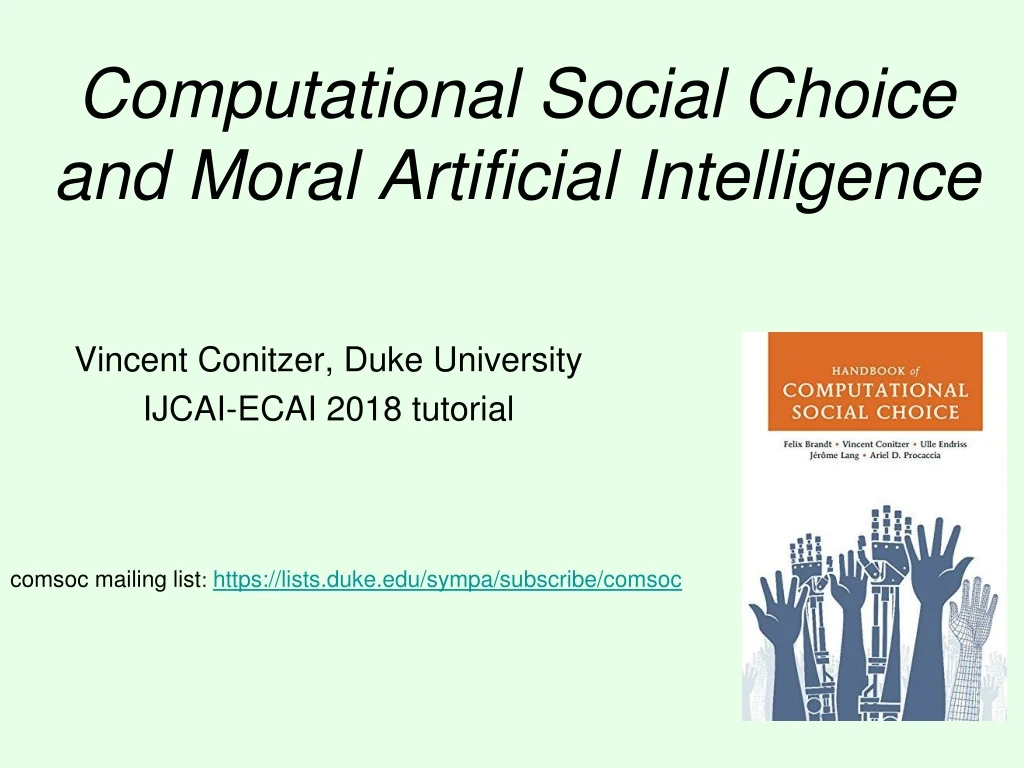
1. Computational Social Choice and Moral Artificial Intelligence Vincent Conitzer, Duke University IJCAI-ECAI 2018 tutorial comsoc mailing list:https://lists.duke.edu/sympa/subscribe/comsoc

2. Lirong Xia (Ph.D. 2011, now at RPI) Markus Brill (postdoc 2013-2015, now at TU Berlin) Rupert Freeman (Ph.D. 2018, joining MSR NYC for postdoc) some slides based on UlleEndriss

3. Voting n voters… … each produce a ranking of m alternatives… … which a social preference function (SPF) maps to one or more aggregate rankings. b≻a≻c a ≻ b ≻ c … or, a social choice function (SCF) just produces one or more winners. a≻c≻b a a≻b ≻c

4. Plurality 1 0 0 b≻a≻c a ≻ b ≻ c a≻c≻b 2 1 0 a≻b ≻c

5. Borda 2 1 0 b≻a≻c a ≻ b ≻ c a≻c≻b 5 3 1 a≻b ≻c

6. Instant runoff voting / single transferable vote (STV) b≻a≻c b≻a a a ≻ b ≻ c a≻c≻b a≻b a a≻b ≻c a a≻b

7. Kemeny b≻a≻c a ≻ b ≻ c a≻c≻b 2 disagreements ↔ 3*3 - 2 = 7 agreements (maximum) a≻b ≻c • Natural interpretation as maximum likelihood estimate of the “correct” ranking [Young 1988, 1995]

8. Pairwise election graphs • Pairwise election between a and b: compare how often a is ranked above b vs. how often b is ranked above a • Graph representation: edge from winner to loser (no edge if tie), weight = margin of victory • E.g., for votes a > b > c > d, c > a > d > b thisgives b a 2 2 2 c d

9. Kemeny on pairwise election graphs • Final ranking = acyclic tournament graph • Edge (a, b) means a ranked above b • Acyclic = no cycles, tournament = edge between every pair • Kemeny ranking seeks to minimize the total weight of the inverted edges Kemeny ranking pairwise election graph 2 2 b a b a 2 4 2 2 10 c d c d 4 (b > d > c > a) • NP-hard even with 4 voters [Dwork et al. 2001] • Integer programs scale reasonably [C., Davenport, Kalagnanam 2006]

10. Ranking Ph.D. applicants (briefly described in C. [2010]) • Input: Rankings of subsets of the (non-eliminated) applicants ≻ ≻ ≻ ≻ • Output: (one) Kemeny ranking of the (non-eliminated) applicants ≻ ≻

11. Choosing a rule • How do we choose a rule from all of these rules? • How do we know that there does not exist another, “perfect” rule? • Let us look at some criteria that we would like our voting rule to satisfy

12. Condorcet criterion • A candidate is the Condorcet winner if it wins all of its pairwise elections • Does not always exist… • … but the Condorcet criterion says that if it does exist, it should win • Many rules do not satisfy this • E.g., for plurality: • b > a > c > d • c > a > b > d • d > a > b > c • a is the Condorcet winner, but it does not win under plurality

13. Consistency (SPF sense) • An SPF f is said to be consistent if the following holds: • Suppose V1 and V2 are two voting profiles (multisets) such that f produces the same ranking on both • Then f should produce the same ranking on their union. • Which of our rules satisfy this?

14. Consistency (SCF sense) • An SCF f is said to be consistent if the following holds: • Suppose V1 and V2 are two voting profiles (multisets) such that f produces the same winner on both • Then f should produce the same winner on their union. • Which of our rules satisfy this? • Consistency properties are closely related to interpretability as MLE of the truth [C., Rognlie, Xia 2009]

15. Some axiomatizations • Theorem[Young 1975]. An SCF is symmetric, consistent, and continuous if and only if it is a positional scoring rule. • Theorem[Young and Levenglick 1978]. An SPF is neutral, consistent, and Condorcet if and only if it is the Kemeny SPF. • Theorem [Freeman, Brill, C. 2014]. An SPF satisfiesindependence of bottom alternatives, consistency at the bottom, independence of clones (& some minor conditions) if and only if it is the STV SPF.

16. Manipulability • Sometimes, a voter is better off revealing her preferences insincerely, AKA manipulating • E.g., plurality • Suppose a voter prefers a > b > c • Also suppose she knows that the other votes are • 2 times b > c > a • 2 times c > a > b • Voting truthfully will lead to a tie between b and c • She would be better off voting, e.g., b > a > c, guaranteeing b wins

17. Gibbard-Satterthwaite impossibility theorem • Suppose there are at least 3 alternatives • There exists no rule that is simultaneously: • non-imposing/onto (for every alternative, there are some votes that would make that alternative win), • nondictatorial (there does not exist a voter such that the rule simply always selects that voter’s first-ranked alternative as the winner), and • nonmanipulable/strategy-proof

18. Single-peaked preferences • Suppose candidates are ordered on a line • Every voter prefers candidates that are closer to her most preferred candidate • Let every voter report only her most preferred candidate (“peak”) • Choose the median voter’s peak as the winner • This will also be the Condorcet winner • Nonmanipulable! Impossibility results do not necessarily hold when the space of preferences is restricted v5 v4 v2 v1 v3 a1 a2 a3 a4 a5

19. Moulin’s characterization • Slight generalization: add phantom voters, then choose the median of real+phantom voters • Theorem[Moulin 1980]. Under single-peaked preferences, an SCF is strategy-proof, Pareto efficient, and anonymous if and only if it is such a generalized median rule. v5 v3 p3 v4 v2 p2 v1 p4 p1 a1 a2 a3 a4 a5

20. Computational hardness as a barrier to manipulation • A (successful) manipulation is a way of misreporting one’s preferences that leads to a better result for oneself • Gibbard-Satterthwaite only tells us that for some instances, successful manipulations exist • It does not say that these manipulations are always easy to find • Do voting rules exist for which manipulations are computationally hard to find?

21. A formal computational problem • The simplest version of the manipulation problem: • CONSTRUCTIVE-MANIPULATION: • We are given a voting rule r, the (unweighted) votes of the other voters, and an alternative p. • We are asked if we can cast our (single) vote to make p win. • E.g., for the Borda rule: • Voter 1 votes A > B > C • Voter 2 votes B > A > C • Voter 3 votes C > A > B • Borda scores are now: A: 4, B: 3, C: 2 • Can we make B win? • Answer: YES. Vote B > C > A (Borda scores: A: 4, B: 5, C: 3)

22. Early research • Theorem. CONSTRUCTIVE-MANIPULATION is NP-complete for the second-order Copeland rule. [Bartholdi, Tovey, Trick 1989] • Second order Copeland = alternative’s score is sum of Copeland scores of alternatives it defeats • Theorem. CONSTRUCTIVE-MANIPULATION is NP-complete for the STV rule. [Bartholdi, Orlin 1991] • Most other rules are easy to manipulate (in P)

23. Ranked pairs rule [Tideman 1987] • Order pairwise elections by decreasing strength of victory • Successively “lock in” results of pairwise elections unless it causes a cycle 6 b a 12 Final ranking: c>a>b>d 4 8 10 c d 2 • Theorem. CONSTRUCTIVE-MANIPULATION is NP-complete for the ranked pairs rule [Xia et al. IJCAI 2009]

24. Many manipulation problems… Table from: C. & Walsh, Barriers to Manipulation, Chapter 6 in Handbook of Computational Social Choice

25. STV manipulation algorithm[C., Sandholm, Lang JACM 2007] Runs in O(((1+√5)/2)m) time (worst case) nobody eliminated yet rescue d don’t rescue d c eliminated d eliminated no choice for manipulator rescue a don’t rescue a b eliminated b eliminated a eliminated no choice for manipulator no choice for manipulator don’t rescue c rescue c d eliminated … … … rescue a don’t rescue a … …

26. Runtime on random votes [Walsh 2011]

27. Fine – how about another rule? • Heuristic algorithms and/or experimental (simulation) evaluation [C. & Sandholm 2006, Procaccia & Rosenschein 2007, Walsh 2011, Davies, Katsirelos, Narodytska, Walsh 2011] • Quantitative versions of Gibbard-Satterthwaite showing that under certain conditions, for some voter, even a random manipulation on a random instance has significant probability of succeeding [Friedgut, Kalai, Nisan 2008; Xia & C. 2008; Dobzinski & Procaccia 2008; Isaksson, Kindler, Mossel 2010; Mossel & Racz 2013] “for a social choice function f on k≥3 alternatives and n voters, which is ϵ-far from the family of nonmanipulable functions, a uniformly chosen voter profile is manipulable with probability at least inverse polynomial in n, k, and ϵ−1.”

28. Judgment aggregation[for an overview, see UlleEndriss’ chapter 17 in the computational social choice handbook] • Three judges have to decide on a case of an alleged breach of contract • They need to decide (a) whether the contract is valid and (b) whether the contract has been breached. • Legal doctrine stipulates that the defendant is liable if and only if (a) and (b) hold.

29. Why is this considered a paradox? • Reason 1:Premise-based procedure and conclusion-based procedure produce different outcomes. • Reason 2: Even though each individual judgment is logically consistent, the majority outcome is not.

30. Distance-based rules • Idea: Find a consistent judgment set that minimizes the “distance” to the profile • Hamming distance between two judgment sets is given by the number of disagreements • distance to a profile given by sum of distances to individual judgment sets in the profile • Two ways to define aggregation rule based on Hamming distance: • minimize Hamming distance to profile • minimize Hamming distance to majority outcome ← generalized Kemeny rule ← generalized Slater rule

31. ɸ1 and ɸ2 are both equivalent to p ∨ (q1∧q2) ∨ (r1∧r2∧r3) Example